Compute Latency
This example demonstrates how to use direct function calls of the low-level TAT-C library to perform latency analysis.
Similar to the Collect Observations and Compute Coverage examples, the first steps are to define the satellites for the mission. This example again uses the NOAA-20 satellite with a two-line elements model from July 2022 and a VIIRS instrument with field of regard computed based on a 834km altitude and 3000km swath width. Points are distributed over the globe with a 5000 km characteristic distance and observations are collected over a 30 day period starting on July 14, 2022 at noon UTC.
from tatc import utils
from tatc.schemas import Instrument, Satellite, TwoLineElements

viirs = Instrument(
    name="VIIRS",
    field_of_regard=utils.swath_width_to_field_of_regard(834000, 3000000),
    req_target_sunlit=True,
)
noaa20 = Satellite(
    name="NOAA 20",
    orbit=TwoLineElements(
        tle=[
            "1 43013U 17073A   22195.78278435  .00000038  00000+0  38919-4 0  9996",
            "2 43013  98.7169 133.9110 0001202  63.8768 296.2532 14.19561306241107",
        ]
    ),
    instruments=[viirs],
)

from tatc.generation import generate_equally_spaced_points

points_df = generate_equally_spaced_points(5000e3)

from tatc.schemas import Point

points = points_df.apply(
    lambda r: Point(id=r.point_id, latitude=r.geometry.y, longitude=r.geometry.x),
    axis=1,
)

from datetime import datetime, timedelta, timezone

start = datetime(year=2022, month=7, day=14, hour=12, tzinfo=timezone.utc)
end = start + timedelta(days=30)

from tatc.analysis import collect_observations
from joblib import Parallel, delayed
import pandas as pd

observations_list = Parallel(n_jobs=-1)(
    delayed(collect_observations)(point, noaa20, start, end) for point in points
)
observations = pd.concat(observations_list, ignore_index=True)
display(observations)
| point_id | geometry | satellite | instrument | start | end | epoch | sat_alt | sat_az | |
|---|---|---|---|---|---|---|---|---|---|
| 0 | 0 | POINT Z (-157.51699 -67.51699 0) | NOAA 20 | VIIRS | 2022-07-26 23:05:45.258746+00:00 | 2022-07-26 23:08:44.580526+00:00 | 2022-07-26 23:07:14.919636+00:00 | 23.232376 | 96.383771 |
| 1 | 0 | POINT Z (-157.51699 -67.51699 0) | NOAA 20 | VIIRS | 2022-07-30 23:30:00.700453+00:00 | 2022-07-30 23:35:11.668269+00:00 | 2022-07-30 23:32:36.184361+00:00 | 29.980441 | 90.571477 |
| 2 | 0 | POINT Z (-157.51699 -67.51699 0) | NOAA 20 | VIIRS | 2022-07-31 01:09:44.380087+00:00 | 2022-07-31 01:17:23.069693+00:00 | 2022-07-31 01:13:33.724890+00:00 | 83.932517 | 71.659563 |
| 3 | 0 | POINT Z (-157.51699 -67.51699 0) | NOAA 20 | VIIRS | 2022-07-31 23:11:40.551119+00:00 | 2022-07-31 23:15:24.047070+00:00 | 2022-07-31 23:13:32.299094500+00:00 | 24.749767 | 94.883549 |
| 4 | 0 | POINT Z (-157.51699 -67.51699 0) | NOAA 20 | VIIRS | 2022-08-01 00:50:55.502645+00:00 | 2022-08-01 00:58:28.482647+00:00 | 2022-08-01 00:54:41.992646+00:00 | 70.126386 | 72.613305 |
| ... | ... | ... | ... | ... | ... | ... | ... | ... | ... |
| 2169 | 31 | POINT Z (157.24514 67.38106 0) | NOAA 20 | VIIRS | 2022-08-12 18:28:51.557986+00:00 | 2022-08-12 18:34:04.353232+00:00 | 2022-08-12 18:31:27.955609+00:00 | 31.258697 | 324.067710 |
| 2170 | 31 | POINT Z (157.24514 67.38106 0) | NOAA 20 | VIIRS | 2022-08-12 21:48:45.630367+00:00 | 2022-08-12 21:49:49.415577+00:00 | 2022-08-12 21:49:17.522972+00:00 | 21.115155 | 12.621024 |
| 2171 | 31 | POINT Z (157.24514 67.38106 0) | NOAA 20 | VIIRS | 2022-08-12 23:25:37.442375+00:00 | 2022-08-12 23:31:05.304568+00:00 | 2022-08-12 23:28:21.373471500+00:00 | 32.779326 | 36.304442 |
| 2172 | 31 | POINT Z (157.24514 67.38106 0) | NOAA 20 | VIIRS | 2022-08-13 01:04:22.215027+00:00 | 2022-08-13 01:11:48.221137+00:00 | 2022-08-13 01:08:05.218082+00:00 | 73.798507 | 55.756224 |
| 2173 | 31 | POINT Z (157.24514 67.38106 0) | NOAA 20 | VIIRS | 2022-08-13 02:45:33.011228+00:00 | 2022-08-13 02:51:56.674083+00:00 | 2022-08-13 02:48:44.842655500+00:00 | 40.285445 | 264.921794 |
2174 rows × 9 columns
Latency analysis measures the interval between observations and downlink to the first ground station. The following specifies a ground station at Hoboken with a 10-degree minimum elevaiton angle for downlink.
from tatc.schemas import GroundStation

hoboken = GroundStation(
    name="Hoboken", latitude=40.74259, longitude=-74.02686, min_elevation_angle=10
)

from tatc.analysis import collect_downlinks

downlinks = collect_downlinks(hoboken, noaa20, start, end)
display(downlinks)
| station | geometry | satellite | start | end | epoch | |
|---|---|---|---|---|---|---|
| 0 | Hoboken | POINT Z (-74.02686 40.74259 0) | NOAA 20 | 2022-07-14 17:12:43.763296+00:00 | 2022-07-14 17:22:57.456044+00:00 | 2022-07-14 17:17:50.609670+00:00 |
| 1 | Hoboken | POINT Z (-74.02686 40.74259 0) | NOAA 20 | 2022-07-14 18:54:04.803537+00:00 | 2022-07-14 19:02:25.062501+00:00 | 2022-07-14 18:58:14.933019+00:00 |
| 2 | Hoboken | POINT Z (-74.02686 40.74259 0) | NOAA 20 | 2022-07-15 05:32:06.654997+00:00 | 2022-07-15 05:39:35.858756+00:00 | 2022-07-15 05:35:51.256876500+00:00 |
| 3 | Hoboken | POINT Z (-74.02686 40.74259 0) | NOAA 20 | 2022-07-15 07:11:08.223574+00:00 | 2022-07-15 07:21:37.089606+00:00 | 2022-07-15 07:16:22.656590+00:00 |
| 4 | Hoboken | POINT Z (-74.02686 40.74259 0) | NOAA 20 | 2022-07-15 16:54:27.877548+00:00 | 2022-07-15 17:03:52.170605+00:00 | 2022-07-15 16:59:10.024076500+00:00 |
| ... | ... | ... | ... | ... | ... | ... |
| 115 | Hoboken | POINT Z (-74.02686 40.74259 0) | NOAA 20 | 2022-08-12 08:28:09.529139+00:00 | 2022-08-12 08:32:42.603014+00:00 | 2022-08-12 08:30:26.066076500+00:00 |
| 116 | Hoboken | POINT Z (-74.02686 40.74259 0) | NOAA 20 | 2022-08-12 16:30:12.255865+00:00 | 2022-08-12 16:37:46.514194+00:00 | 2022-08-12 16:33:59.385029500+00:00 |
| 117 | Hoboken | POINT Z (-74.02686 40.74259 0) | NOAA 20 | 2022-08-12 18:08:28.080213+00:00 | 2022-08-12 18:19:02.956149+00:00 | 2022-08-12 18:13:45.518181+00:00 |
| 118 | Hoboken | POINT Z (-74.02686 40.74259 0) | NOAA 20 | 2022-08-13 06:26:51.204464+00:00 | 2022-08-13 06:37:31.285805+00:00 | 2022-08-13 06:32:11.245134500+00:00 |
| 119 | Hoboken | POINT Z (-74.02686 40.74259 0) | NOAA 20 | 2022-08-13 08:08:18.072998+00:00 | 2022-08-13 08:15:29.539014+00:00 | 2022-08-13 08:11:53.806006+00:00 |
120 rows × 6 columns
Finally, latencies are computed by comparing the observations and downlink opportunities.
from tatc.analysis import compute_latencies

latencies = compute_latencies(observations, downlinks)
display(latencies)
| point_id | geometry | satellite | instrument | sat_alt | sat_az | station | downlinked | latency | observed | |
|---|---|---|---|---|---|---|---|---|---|---|
| 0 | 20 | POINT Z (22.34708 22.41505 0) | NOAA 20 | VIIRS | 46.686116 | 260.777813 | Hoboken | 2022-07-14 17:17:50.609670+00:00 | 0 days 05:10:34.144994500 | 2022-07-14 12:07:16.464675500+00:00 |
| 1 | 28 | POINT Z (22.34708 67.38106 0) | NOAA 20 | VIIRS | 29.024717 | 271.880297 | Hoboken | 2022-07-14 17:17:50.609670+00:00 | 0 days 04:57:46.494320 | 2022-07-14 12:20:04.115350+00:00 |
| 2 | 27 | POINT Z (-22.61894 67.38106 0) | NOAA 20 | VIIRS | 48.704552 | 49.346995 | Hoboken | 2022-07-14 17:17:50.609670+00:00 | 0 days 04:56:13.129769 | 2022-07-14 12:21:37.479901+00:00 |
| 3 | 25 | POINT Z (-112.55097 67.38106 0) | NOAA 20 | VIIRS | 31.323022 | 324.299192 | Hoboken | 2022-07-14 17:17:50.609670+00:00 | 0 days 04:47:32.626919500 | 2022-07-14 12:30:17.982750500+00:00 |
| 4 | 24 | POINT Z (-157.51699 67.38106 0) | NOAA 20 | VIIRS | 55.694847 | 103.325667 | Hoboken | 2022-07-14 17:17:50.609670+00:00 | 0 days 04:44:55.809464 | 2022-07-14 12:32:54.800206+00:00 |
| ... | ... | ... | ... | ... | ... | ... | ... | ... | ... | ... |
| 2169 | 26 | POINT Z (-67.58495 67.38106 0) | NOAA 20 | VIIRS | 28.848897 | 327.376449 | None | NaT | NaT | 2022-08-13 09:44:37.403851500+00:00 |
| 2170 | 5 | POINT Z (67.3131 -67.51699 0) | NOAA 20 | VIIRS | 78.725002 | 245.320118 | None | NaT | NaT | 2022-08-13 10:37:41.608547500+00:00 |
| 2171 | 20 | POINT Z (22.34708 22.41505 0) | NOAA 20 | VIIRS | 35.605265 | 70.967792 | None | NaT | NaT | 2022-08-13 11:04:24.936363+00:00 |
| 2172 | 28 | POINT Z (22.34708 67.38106 0) | NOAA 20 | VIIRS | 56.654314 | 258.438321 | None | NaT | NaT | 2022-08-13 11:16:22.849990500+00:00 |
| 2173 | 27 | POINT Z (-22.61894 67.38106 0) | NOAA 20 | VIIRS | 31.043210 | 33.884307 | None | NaT | NaT | 2022-08-13 11:19:02.608528500+00:00 |
2174 rows × 10 columns
Similar to Coverage Analysis, latency analysis can also be reduced to compute descriptive statistics for each observation point.
from tatc.analysis import reduce_latencies

reduced_results = reduce_latencies(latencies)
display(reduced_results)
| point_id | geometry | latency | samples | |
|---|---|---|---|---|
| 0 | 0 | POINT Z (-157.51699 -67.51699 0) | 0 days 05:10:59.268689 | 31 |
| 1 | 1 | POINT Z (-112.55097 -67.51699 0) | 0 days 08:14:18.836280 | 31 |
| 2 | 2 | POINT Z (-67.58495 -67.51699 0) | 0 days 04:21:48.654757 | 30 |
| 3 | 3 | POINT Z (-22.61894 -67.51699 0) | 0 days 01:17:44.394353 | 31 |
| 4 | 4 | POINT Z (22.34708 -67.51699 0) | 0 days 04:08:15.422021 | 31 |
| 5 | 5 | POINT Z (67.3131 -67.51699 0) | 0 days 08:42:06.877307 | 31 |
| 6 | 6 | POINT Z (112.27912 -67.51699 0) | 0 days 02:43:07.838991 | 33 |
| 7 | 7 | POINT Z (157.24514 -67.51699 0) | 0 days 02:19:26.312887 | 34 |
| 8 | 8 | POINT Z (-157.51699 -22.55097 0) | 0 days 05:44:31.317841 | 34 |
| 9 | 9 | POINT Z (-112.55097 -22.55097 0) | 0 days 08:37:46.021444 | 34 |
| 10 | 10 | POINT Z (-67.58495 -22.55097 0) | 0 days 00:17:46.170450 | 32 |
| 11 | 11 | POINT Z (-22.61894 -22.55097 0) | 0 days 01:35:26.242661 | 32 |
| 12 | 12 | POINT Z (22.34708 -22.55097 0) | 0 days 04:33:05.882867 | 32 |
| 13 | 13 | POINT Z (67.3131 -22.55097 0) | 0 days 09:05:11.024889 | 34 |
| 14 | 14 | POINT Z (112.27912 -22.55097 0) | 0 days 00:45:24.121858 | 32 |
| 15 | 15 | POINT Z (157.24514 -22.55097 0) | 0 days 02:52:47.346982 | 32 |
| 16 | 16 | POINT Z (-157.51699 22.41505 0) | 0 days 06:21:54.644226 | 32 |
| 17 | 17 | POINT Z (-112.55097 22.41505 0) | 0 days 09:24:22.656684 | 34 |
| 18 | 18 | POINT Z (-67.58495 22.41505 0) | 0 days 06:12:15.863428 | 32 |
| 19 | 19 | POINT Z (-22.61894 22.41505 0) | 0 days 02:11:37.441686 | 34 |
| 20 | 20 | POINT Z (22.34708 22.41505 0) | 0 days 06:27:50.003063 | 34 |
| 21 | 21 | POINT Z (67.3131 22.41505 0) | 0 days 07:34:34.545599 | 32 |
| 22 | 22 | POINT Z (112.27912 22.41505 0) | 0 days 00:32:56.099903 | 34 |
| 23 | 23 | POINT Z (157.24514 22.41505 0) | 0 days 03:11:43.033986 | 32 |
| 24 | 24 | POINT Z (-157.51699 67.38106 0) | 0 days 05:48:32.308626 | 173 |
| 25 | 25 | POINT Z (-112.55097 67.38106 0) | 0 days 06:31:10.233941 | 173 |
| 26 | 26 | POINT Z (-67.58495 67.38106 0) | 0 days 04:58:06.133920 | 171 |
| 27 | 27 | POINT Z (-22.61894 67.38106 0) | 0 days 03:01:50.017806 | 176 |
| 28 | 28 | POINT Z (22.34708 67.38106 0) | 0 days 04:34:58.875476 | 174 |
| 29 | 29 | POINT Z (67.3131 67.38106 0) | 0 days 04:11:56.901332 | 174 |
| 30 | 30 | POINT Z (112.27912 67.38106 0) | 0 days 04:35:16.325513 | 177 |
| 31 | 31 | POINT Z (157.24514 67.38106 0) | 0 days 05:24:20.336656 | 178 |
Finally, GeoPlot can visualize the geospatial data.
import matplotlib.pyplot as plt
import cartopy.crs as ccrs

reduced_results["latency_hr"] = reduced_results.latency / timedelta(hours=1)

fig, ax = plt.subplots(figsize=(8, 6), subplot_kw={"projection": ccrs.PlateCarree()})
reduced_results.plot(
    column="latency_hr",
    legend=True,
    legend_kwds={"label": "Latency (hr)", "orientation": "horizontal"},
    ax=ax,
    transform=ccrs.PlateCarree()
)
ax.coastlines()
ax.set_global()
plt.show()
Similar to Coverage Analysis, cells can also be used to aggregate descriptive statistics. Note that, when working on the reduced results, the revisit aggregation function must perform a weighted average based on the number of samples for each point.
from tatc.generation.cells import generate_equally_spaced_cells

cells_df = generate_equally_spaced_cells(5000e3)

import numpy as np

grid_results = (
    cells_df.sjoin(reduced_results, how="inner", predicate="contains")
    .dissolve(
        by="cell_id",
        aggfunc={
            "samples": "sum",
            "latency_hr": lambda r: np.average(
                r, weights=reduced_results.loc[r.index, "samples"]
            ),
        },
    )
    .reset_index()
)
display(grid_results)
| cell_id | geometry | samples | latency_hr | |
|---|---|---|---|---|
| 0 | 0 | POLYGON Z ((-135.03398 -90 0, -135.03398 -45.0... | 31 | 5.183130 |
| 1 | 1 | POLYGON Z ((-90.06796 -90 0, -90.06796 -45.033... | 31 | 8.238566 |
| 2 | 2 | POLYGON Z ((-45.10194 -90 0, -45.10194 -45.033... | 30 | 4.363515 |
| 3 | 3 | POLYGON Z ((-0.13593 -90 0, -0.13593 -45.03398... | 31 | 1.295665 |
| 4 | 4 | POLYGON Z ((44.83009 -90 0, 44.83009 -45.03398... | 31 | 4.137617 |
| 5 | 5 | POLYGON Z ((89.79611 -90 0, 89.79611 -45.03398... | 31 | 8.701910 |
| 6 | 6 | POLYGON Z ((134.76213 -90 0, 134.76213 -45.033... | 33 | 2.718844 |
| 7 | 7 | POLYGON Z ((179.72815 -90 0, 179.72815 -45.033... | 34 | 2.323976 |
| 8 | 8 | POLYGON Z ((-135.03398 -45.03398 0, -135.03398... | 34 | 5.742033 |
| 9 | 9 | POLYGON Z ((-90.06796 -45.03398 0, -90.06796 -... | 34 | 8.629450 |
| 10 | 10 | POLYGON Z ((-45.10194 -45.03398 0, -45.10194 -... | 32 | 0.296158 |
| 11 | 11 | POLYGON Z ((-0.13593 -45.03398 0, -0.13593 -0.... | 32 | 1.590623 |
| 12 | 12 | POLYGON Z ((44.83009 -45.03398 0, 44.83009 -0.... | 32 | 4.551634 |
| 13 | 13 | POLYGON Z ((89.79611 -45.03398 0, 89.79611 -0.... | 34 | 9.086396 |
| 14 | 14 | POLYGON Z ((134.76213 -45.03398 0, 134.76213 -... | 32 | 0.756701 |
| 15 | 15 | POLYGON Z ((179.72815 -45.03398 0, 179.72815 -... | 32 | 2.879819 |
| 16 | 16 | POLYGON Z ((-135.03398 -0.06796 0, -135.03398 ... | 32 | 6.365179 |
| 17 | 17 | POLYGON Z ((-90.06796 -0.06796 0, -90.06796 44... | 34 | 9.406294 |
| 18 | 18 | POLYGON Z ((-45.10194 -0.06796 0, -45.10194 44... | 32 | 6.204407 |
| 19 | 19 | POLYGON Z ((-0.13593 -0.06796 0, -0.13593 44.8... | 34 | 2.193734 |
| 20 | 20 | POLYGON Z ((44.83009 -0.06796 0, 44.83009 44.8... | 34 | 6.463890 |
| 21 | 21 | POLYGON Z ((89.79611 -0.06796 0, 89.79611 44.8... | 32 | 7.576263 |
| 22 | 22 | POLYGON Z ((134.76213 -0.06796 0, 134.76213 44... | 34 | 0.548917 |
| 23 | 23 | POLYGON Z ((179.72815 -0.06796 0, 179.72815 44... | 32 | 3.195287 |
| 24 | 24 | POLYGON Z ((-135.03398 44.89806 0, -135.03398 ... | 173 | 5.808975 |
| 25 | 25 | POLYGON Z ((-90.06796 44.89806 0, -90.06796 89... | 173 | 6.519509 |
| 26 | 26 | POLYGON Z ((-45.10194 44.89806 0, -45.10194 89... | 171 | 4.968371 |
| 27 | 27 | POLYGON Z ((-0.13593 44.89806 0, -0.13593 89.8... | 176 | 3.030561 |
| 28 | 28 | POLYGON Z ((44.83009 44.89806 0, 44.83009 89.8... | 174 | 4.583021 |
| 29 | 29 | POLYGON Z ((89.79611 44.89806 0, 89.79611 89.8... | 174 | 4.199139 |
| 30 | 30 | POLYGON Z ((134.76213 44.89806 0, 134.76213 89... | 177 | 4.587868 |
| 31 | 31 | POLYGON Z ((179.72815 44.89806 0, 179.72815 89... | 178 | 5.405649 |
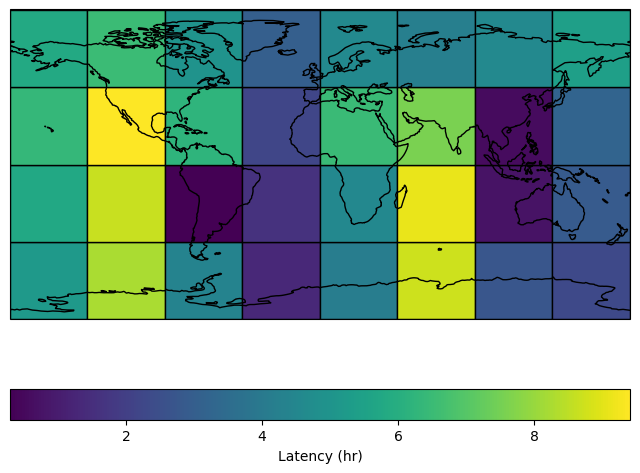
Finally, plotting can illustrate the latency over global regions.
import matplotlib.pyplot as plt
import cartopy.crs as ccrs

fig, ax = plt.subplots(figsize=(8, 6), subplot_kw={"projection": ccrs.PlateCarree()})
grid_results.plot(
    column="latency_hr",
    cmap="viridis",
    edgecolor="k",
    legend=True,
    legend_kwds={"label": "Latency (hr)", "orientation": "horizontal"},
    ax=ax,
)
ax.coastlines()
ax.set_global()
plt.show()