Collect Orbit and Ground Track
This example demonstrates how to use direct function calls of the low-level TAT-C library to collect satellite orbit and ground tracks.
Similar to the Collect Observations example, the first steps are to define the satellites for the mission. This example again uses the NOAA-20 satellite with a two-line elements model from July 2022 and a VIIRS instrument with field of regard computed based on a 834km altitude and 3000km swath width. This example also adds an operational requirement that targets must be sunlit for valid observations.
from tatc import utils
from tatc.schemas import Instrument, Satellite, TwoLineElements

viirs = Instrument(
    name="VIIRS",
    field_of_regard=utils.swath_width_to_field_of_regard(834000, 3000000),
    req_target_sunlit=True,
)
noaa20 = Satellite(
    name="NOAA 20",
    orbit=TwoLineElements(
        tle=[
            "1 43013U 17073A   22195.78278435  .00000038  00000+0  38919-4 0  9996",
            "2 43013  98.7169 133.9110 0001202  63.8768 296.2532 14.19561306241107",
        ]
    ),
    instruments=[viirs],
)
Next, we can identify the starting and ending times and sampling interval of a sample mission period. The starting time is noon UTC on July 14, 2022 and the ending time is 2 hours later (noon UTC on July 16, 2022). The sampling frequency is set to 2 minutes.
from datetime import datetime, timedelta, timezone
import pandas as pd

start = datetime(year=2022, month=7, day=14, hour=12, tzinfo=timezone.utc)
end = start + timedelta(hours=2)
delta = timedelta(minutes=2)
times = pd.date_range(start, end, freq=delta)
display(times)
DatetimeIndex(['2022-07-14 12:00:00+00:00', '2022-07-14 12:02:00+00:00',
               '2022-07-14 12:04:00+00:00', '2022-07-14 12:06:00+00:00',
               '2022-07-14 12:08:00+00:00', '2022-07-14 12:10:00+00:00',
               '2022-07-14 12:12:00+00:00', '2022-07-14 12:14:00+00:00',
               '2022-07-14 12:16:00+00:00', '2022-07-14 12:18:00+00:00',
               '2022-07-14 12:20:00+00:00', '2022-07-14 12:22:00+00:00',
               '2022-07-14 12:24:00+00:00', '2022-07-14 12:26:00+00:00',
               '2022-07-14 12:28:00+00:00', '2022-07-14 12:30:00+00:00',
               '2022-07-14 12:32:00+00:00', '2022-07-14 12:34:00+00:00',
               '2022-07-14 12:36:00+00:00', '2022-07-14 12:38:00+00:00',
               '2022-07-14 12:40:00+00:00', '2022-07-14 12:42:00+00:00',
               '2022-07-14 12:44:00+00:00', '2022-07-14 12:46:00+00:00',
               '2022-07-14 12:48:00+00:00', '2022-07-14 12:50:00+00:00',
               '2022-07-14 12:52:00+00:00', '2022-07-14 12:54:00+00:00',
               '2022-07-14 12:56:00+00:00', '2022-07-14 12:58:00+00:00',
               '2022-07-14 13:00:00+00:00', '2022-07-14 13:02:00+00:00',
               '2022-07-14 13:04:00+00:00', '2022-07-14 13:06:00+00:00',
               '2022-07-14 13:08:00+00:00', '2022-07-14 13:10:00+00:00',
               '2022-07-14 13:12:00+00:00', '2022-07-14 13:14:00+00:00',
               '2022-07-14 13:16:00+00:00', '2022-07-14 13:18:00+00:00',
               '2022-07-14 13:20:00+00:00', '2022-07-14 13:22:00+00:00',
               '2022-07-14 13:24:00+00:00', '2022-07-14 13:26:00+00:00',
               '2022-07-14 13:28:00+00:00', '2022-07-14 13:30:00+00:00',
               '2022-07-14 13:32:00+00:00', '2022-07-14 13:34:00+00:00',
               '2022-07-14 13:36:00+00:00', '2022-07-14 13:38:00+00:00',
               '2022-07-14 13:40:00+00:00', '2022-07-14 13:42:00+00:00',
               '2022-07-14 13:44:00+00:00', '2022-07-14 13:46:00+00:00',
               '2022-07-14 13:48:00+00:00', '2022-07-14 13:50:00+00:00',
               '2022-07-14 13:52:00+00:00', '2022-07-14 13:54:00+00:00',
               '2022-07-14 13:56:00+00:00', '2022-07-14 13:58:00+00:00',
               '2022-07-14 14:00:00+00:00'],
              dtype='datetime64[ns, UTC]', freq='2min')
The collect_orbit_track method can be called generates points representing the orbital motion of the satellite during the mission. Results are formatted as a flat GeoDataFrame which is similar to a regular pandas DataFrame with a geospatial column labeled geometry. Other columns:
time: sample timeswath_width: projected instrument swath width (m) based on the specified field of regardvalid_obs: boolean whether the observation is “valid” given instrument operational requirements (e.g., sunlit target)
from tatc.analysis import collect_orbit_track

results = collect_orbit_track(noaa20, times)
display(results)
| time | satellite | instrument | swath_width | valid_obs | geometry | |
|---|---|---|---|---|---|---|
| 0 | 2022-07-14 12:00:00+00:00 | NOAA 20 | VIIRS | 2.979477e+06 | True | POINT Z (37.6979 -4.30588 829604.57272) |
| 1 | 2022-07-14 12:02:00+00:00 | NOAA 20 | VIIRS | 2.974766e+06 | True | POINT Z (36.12013 2.75031 828593.05309) |
| 2 | 2022-07-14 12:04:00+00:00 | NOAA 20 | VIIRS | 2.972688e+06 | True | POINT Z (34.52934 9.80636 828146.68837) |
| 3 | 2022-07-14 12:06:00+00:00 | NOAA 20 | VIIRS | 2.973169e+06 | True | POINT Z (32.89116 16.85703 828250.04018) |
| 4 | 2022-07-14 12:08:00+00:00 | NOAA 20 | VIIRS | 2.975986e+06 | True | POINT Z (31.16516 23.89678 828855.11416) |
| ... | ... | ... | ... | ... | ... | ... |
| 56 | 2022-07-14 13:52:00+00:00 | NOAA 20 | VIIRS | 2.982254e+06 | True | POINT Z (3.4244 32.68312 830200.45961) |
| 57 | 2022-07-14 13:54:00+00:00 | NOAA 20 | VIIRS | 2.988873e+06 | True | POINT Z (1.27216 39.67388 831619.33214) |
| 58 | 2022-07-14 13:56:00+00:00 | NOAA 20 | VIIRS | 2.996330e+06 | True | POINT Z (-1.25039 46.62707 833215.3123) |
| 59 | 2022-07-14 13:58:00+00:00 | NOAA 20 | VIIRS | 3.004037e+06 | True | POINT Z (-4.366 53.525 834862.31502) |
| 60 | 2022-07-14 14:00:00+00:00 | NOAA 20 | VIIRS | 3.011412e+06 | True | POINT Z (-8.49191 60.33504 836435.88815) |
61 rows × 6 columns
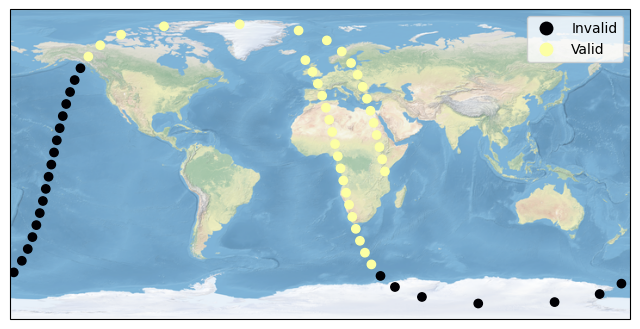
The results can be visualized using a plot.
import matplotlib.pyplot as plt
import cartopy.crs as ccrs

results["valid"] = results.apply(
    lambda r: "Valid" if r.valid_obs else "Invalid", axis=1
)

fig, ax = plt.subplots(figsize=(8, 5), subplot_kw={"projection": ccrs.PlateCarree()})

results.plot(
    column="valid",
    legend=True,
    cmap="inferno",
    ax=ax,
    transform=ccrs.PlateCarree()
)
ax.stock_img()
ax.set_global()
plt.show()
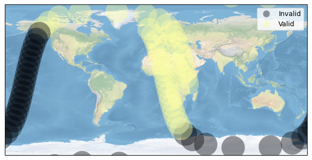
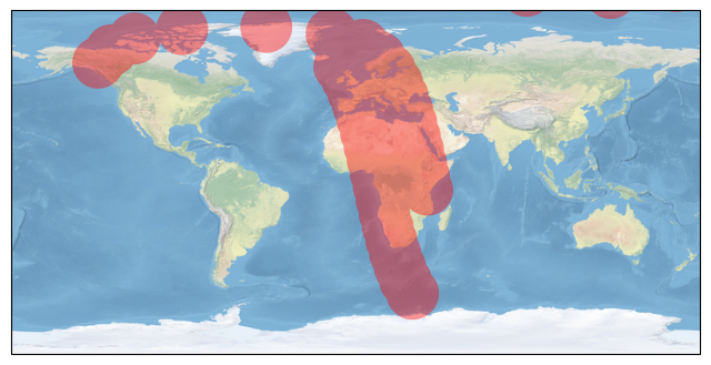
The collect_ground_track method projects a ground track using knowledge of the instrument. The default setting applies a buffer equivalent to the half swath width to each point in the EPSG:4087 World Equidistant Cylindrical coordinate system. The resulting Polygon geometry is automatically split into a MultiPolygon when crossing the anti-meridian (+/- 180 degrees longitude) and/or the north/south pole (+/- 90 degrees latitude).
from tatc.analysis import collect_ground_track

results = collect_ground_track(noaa20, times)
display(results)
| time | satellite | instrument | swath_width | valid_obs | geometry | |
|---|---|---|---|---|---|---|
| 0 | 2022-07-14 12:00:00+00:00 | NOAA 20 | VIIRS | 2.979477e+06 | True | POLYGON Z ((51.08044 -4.30588 0, 51.016 -5.617... |
| 1 | 2022-07-14 12:02:00+00:00 | NOAA 20 | VIIRS | 2.974766e+06 | True | POLYGON Z ((49.48151 2.75031 0, 49.41718 1.440... |
| 2 | 2022-07-14 12:04:00+00:00 | NOAA 20 | VIIRS | 2.972688e+06 | True | POLYGON Z ((47.88139 9.80636 0, 47.8171 8.4976... |
| 3 | 2022-07-14 12:06:00+00:00 | NOAA 20 | VIIRS | 2.973169e+06 | True | POLYGON Z ((46.24537 16.85703 0, 46.18107 15.5... |
| 4 | 2022-07-14 12:08:00+00:00 | NOAA 20 | VIIRS | 2.975986e+06 | True | POLYGON Z ((44.53202 23.89678 0, 44.46766 22.5... |
| ... | ... | ... | ... | ... | ... | ... |
| 56 | 2022-07-14 13:52:00+00:00 | NOAA 20 | VIIRS | 2.982254e+06 | True | POLYGON Z ((16.81942 32.68312 0, 16.75492 31.3... |
| 57 | 2022-07-14 13:54:00+00:00 | NOAA 20 | VIIRS | 2.988873e+06 | True | POLYGON Z ((14.69691 39.67388 0, 14.63227 38.3... |
| 58 | 2022-07-14 13:56:00+00:00 | NOAA 20 | VIIRS | 2.996330e+06 | True | POLYGON Z ((12.20786 46.62707 0, 12.14305 45.3... |
| 59 | 2022-07-14 13:58:00+00:00 | NOAA 20 | VIIRS | 3.004037e+06 | True | POLYGON Z ((9.12686 53.525 0, 9.06189 52.20247... |
| 60 | 2022-07-14 14:00:00+00:00 | NOAA 20 | VIIRS | 3.011412e+06 | True | POLYGON Z ((5.03408 60.33504 0, 4.96895 59.009... |
61 rows × 6 columns
While fast, the EPSG:4087 coordinate reference frame is not accurate near the poles, as seen in the plot below.
import matplotlib.pyplot as plt
import cartopy.crs as ccrs

results["valid"] = results.apply(
    lambda r: "Valid" if r.valid_obs else "Invalid", axis=1
)

fig, ax = plt.subplots(figsize=(8, 5), subplot_kw={"projection": ccrs.PlateCarree()})

results.plot(
    column="valid",
    edgecolor="none",
    alpha=0.4,
    legend=True,
    cmap="inferno",
    ax=ax,
    transform=ccrs.PlateCarree()
)
ax.stock_img()
ax.set_global()
plt.show()
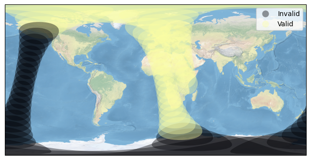
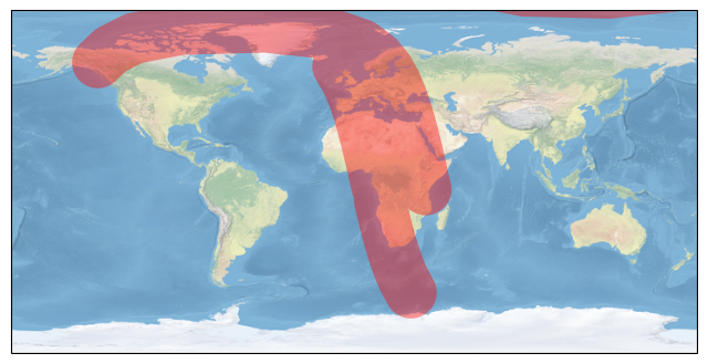
Alternatively, setting crs="utm" uses the Universal Transverse Mercator (UTM) coordinate reference system to more accurately project swath width near the poles. Note that UTM does not cover the regions above 84 degrees or below -80 degrees latitude. These regions instead use the Unified Polar Stereographic (UPS) CRS; however, with poor performance close to the transition point between zones.
import matplotlib.pyplot as plt
import cartopy.crs as ccrs

results = collect_ground_track(noaa20, times, crs="utm")

results["valid"] = results.apply(
    lambda r: "Valid" if r.valid_obs else "Invalid", axis=1
)

fig, ax = plt.subplots(figsize=(8, 5), subplot_kw={"projection": ccrs.PlateCarree()})

results.plot(
    column="valid",
    edgecolor="none",
    alpha=0.4,
    legend=True,
    cmap="inferno",
    ax=ax,
    transform=ccrs.PlateCarree()
)
ax.stock_img()
ax.set_global()
plt.show()
As of TAT-C 3.4.0, the option `spice’ uses an interace to JPL SPICE to quickly and accurately compute ground tracks.
import matplotlib.pyplot as plt
import cartopy.crs as ccrs

results = collect_ground_track(noaa20, times, crs="spice")

results["valid"] = results.apply(
    lambda r: "Valid" if r.valid_obs else "Invalid", axis=1
)

fig, ax = plt.subplots(figsize=(8, 5), subplot_kw={"projection": ccrs.PlateCarree()})

results.plot(
    column="valid",
    edgecolor="none",
    alpha=0.4,
    legend=True,
    cmap="inferno",
    ax=ax,
    transform=ccrs.PlateCarree()
)
ax.stock_img()
ax.set_global()
plt.show()

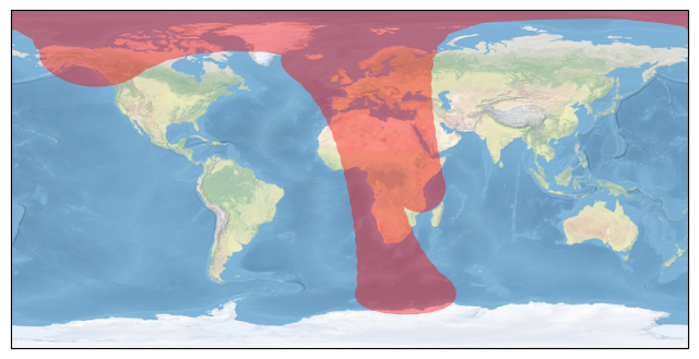
The results can also be processed using compute_ground_track to dissolve geometries.
from tatc.analysis import compute_ground_track

import matplotlib.pyplot as plt
import cartopy.crs as ccrs
import time

t = time.time()
results = compute_ground_track(noaa20, times, method="point")
print(f"Point method (EPSG:4087) completed in {time.time() - t:.2f} seconds")
fig, ax = plt.subplots(figsize=(8, 5), subplot_kw={"projection": ccrs.PlateCarree()})
ax = results.plot(facecolor="r", edgecolor="none", alpha=0.4, zorder=1, ax=ax, transform=ccrs.PlateCarree())
ax.stock_img()
ax.set_global()
plt.show()

t = time.time()
results = compute_ground_track(noaa20, times, crs="utm", method="point")
print(f"Point method (UTM CRS) completed in {time.time() - t:.2f} seconds")
fig, ax = plt.subplots(figsize=(8, 5), subplot_kw={"projection": ccrs.PlateCarree()})
ax = results.plot(facecolor="r", edgecolor="none", alpha=0.4, zorder=1, ax=ax, transform=ccrs.PlateCarree())
ax.stock_img()
ax.set_global()
plt.show()

t = time.time()
results = compute_ground_track(noaa20, times, method="line")
print(f"Line method (EPSG:4087) completed in {time.time() - t:.2f} seconds")
fig, ax = plt.subplots(figsize=(8, 5), subplot_kw={"projection": ccrs.PlateCarree()})
ax = results.plot(facecolor="r", edgecolor="none", alpha=0.4, zorder=1, ax=ax, transform=ccrs.PlateCarree())
ax.stock_img()
ax.set_global()
plt.show()

t = time.time()
results = compute_ground_track(noaa20, times, crs="spice", method="point")
print(f"Point method (SPICE) completed in {time.time() - t:.2f} seconds")
fig, ax = plt.subplots(figsize=(8, 5), subplot_kw={"projection": ccrs.PlateCarree()})
ax = results.plot(facecolor="r", edgecolor="none", alpha=0.4, zorder=1, ax=ax, transform=ccrs.PlateCarree())
ax.stock_img()
ax.set_global()
plt.show()
Point method (EPSG:4087) completed in 0.21 seconds
Point method (UTM CRS) completed in 2.50 seconds

Line method (EPSG:4087) completed in 0.21 seconds
Point method (SPICE) completed in 0.67 seconds