Compute Coverage
This example demonstrates how to use direct function calls of the low-level TAT-C library to perform coverage analysis over a region of interest.
Similar to the Collect Observations example, the first steps are to define the satellites for the mission. This example again uses the NOAA-20 satellite with a two-line elements model from July 2022 and a VIIRS instrument with field of regard computed based on a 834km altitude and 3000km swath width.
from tatc import utils
from tatc.schemas import Instrument, Satellite, TwoLineElements

viirs = Instrument(
    name="VIIRS",
    field_of_regard=utils.swath_width_to_field_of_regard(834000, 3000000),
)
noaa20 = Satellite(
    name="NOAA 20",
    orbit=TwoLineElements(
        tle=[
            "1 43013U 17073A   22195.78278435  .00000038  00000+0  38919-4 0  9996",
            "2 43013  98.7169 133.9110 0001202  63.8768 296.2532 14.19561306241107",
        ]
    ),
    instruments=[viirs],
)
The mission considers a 30-day integration period starting at noon UTC on July 14, 2022.
from datetime import datetime, timedelta, timezone

start = datetime(year=2022, month=7, day=14, hour=12, tzinfo=timezone.utc)
end = start + timedelta(days=30)
Coverage analyses typically compute metrics over a spatial region. The generate_equally_spaced_points method in TAT-C distributes sample points over a uniform latitude-longitude grid, scaled based on a characteristic distance, set to 5000 km in this example.
from tatc.generation import generate_equally_spaced_points

points_df = generate_equally_spaced_points(5000e3)
display(points_df)
| point_id | geometry | |
|---|---|---|
| 0 | 0 | POINT Z (-157.51699 -67.51699 0) |
| 1 | 1 | POINT Z (-112.55097 -67.51699 0) |
| 2 | 2 | POINT Z (-67.58495 -67.51699 0) |
| 3 | 3 | POINT Z (-22.61894 -67.51699 0) |
| 4 | 4 | POINT Z (22.34708 -67.51699 0) |
| 5 | 5 | POINT Z (67.3131 -67.51699 0) |
| 6 | 6 | POINT Z (112.27912 -67.51699 0) |
| 7 | 7 | POINT Z (157.24514 -67.51699 0) |
| 8 | 8 | POINT Z (-157.51699 -22.55097 0) |
| 9 | 9 | POINT Z (-112.55097 -22.55097 0) |
| 10 | 10 | POINT Z (-67.58495 -22.55097 0) |
| 11 | 11 | POINT Z (-22.61894 -22.55097 0) |
| 12 | 12 | POINT Z (22.34708 -22.55097 0) |
| 13 | 13 | POINT Z (67.3131 -22.55097 0) |
| 14 | 14 | POINT Z (112.27912 -22.55097 0) |
| 15 | 15 | POINT Z (157.24514 -22.55097 0) |
| 16 | 16 | POINT Z (-157.51699 22.41505 0) |
| 17 | 17 | POINT Z (-112.55097 22.41505 0) |
| 18 | 18 | POINT Z (-67.58495 22.41505 0) |
| 19 | 19 | POINT Z (-22.61894 22.41505 0) |
| 20 | 20 | POINT Z (22.34708 22.41505 0) |
| 21 | 21 | POINT Z (67.3131 22.41505 0) |
| 22 | 22 | POINT Z (112.27912 22.41505 0) |
| 23 | 23 | POINT Z (157.24514 22.41505 0) |
| 24 | 24 | POINT Z (-157.51699 67.38106 0) |
| 25 | 25 | POINT Z (-112.55097 67.38106 0) |
| 26 | 26 | POINT Z (-67.58495 67.38106 0) |
| 27 | 27 | POINT Z (-22.61894 67.38106 0) |
| 28 | 28 | POINT Z (22.34708 67.38106 0) |
| 29 | 29 | POINT Z (67.3131 67.38106 0) |
| 30 | 30 | POINT Z (112.27912 67.38106 0) |
| 31 | 31 | POINT Z (157.24514 67.38106 0) |
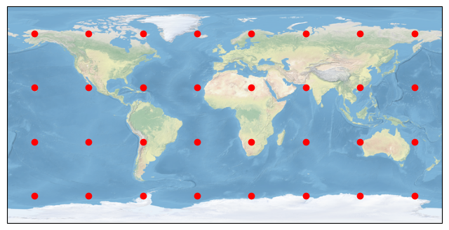
The resulting 32 points are distributed over the globe.
import matplotlib.pyplot as plt
import cartopy.crs as ccrs

fig, ax = plt.subplots(figsize=(8, 5), subplot_kw={"projection": ccrs.PlateCarree()})

points_df.plot(color="red", ax=ax, transform=ccrs.PlateCarree())
ax.stock_img()
ax.set_global()
As the TAT-C analysis functions require points specified in the TAT-C format, rather than a data frame, it is often convenient to convert and store the points in a separate list.
from tatc.schemas import Point

points = points_df.apply(
    lambda r: Point(id=r.point_id, latitude=r.geometry.y, longitude=r.geometry.x),
    axis=1,
)
The collect_observations method can be called either using sequential or parallel computation (using joblib). While there is some overhead associated with parallel computation, it is usually faster on modern multi-core machines.
from tatc.analysis import collect_observations

import time

t = time.time()
results_list = [
    collect_observations(point, noaa20, start, end) for point in points
]
print(f"Sequential computation completed in {time.time() - t:.2f} seconds")
Sequential computation completed in 6.25 seconds
from tatc.analysis import collect_observations

import time
from joblib import Parallel, delayed

t = time.time()
results_list = Parallel(n_jobs=-1)(
    delayed(collect_observations)(point, noaa20, start, end) for point in points
)
print(f"Parallel computation completed in {time.time() - t:.2f} seconds")
Parallel computation completed in 5.86 seconds
Next, we concatenate the results into a single data frame.
import pandas as pd

results = pd.concat(results_list, ignore_index=True)
display(results)
| point_id | geometry | satellite | instrument | start | end | epoch | sat_alt | sat_az | |
|---|---|---|---|---|---|---|---|---|---|
| 0 | 0 | POINT Z (-157.51699 -67.51699 0) | NOAA 20 | VIIRS | 2022-07-14 23:30:13.626441+00:00 | 2022-07-14 23:35:24.594257+00:00 | 2022-07-14 23:32:49.110349+00:00 | 30.035469 | 90.529297 |
| 1 | 0 | POINT Z (-157.51699 -67.51699 0) | NOAA 20 | VIIRS | 2022-07-15 01:09:57.306075+00:00 | 2022-07-15 01:17:35.995681+00:00 | 2022-07-15 01:13:46.650878+00:00 | 84.027751 | 71.150137 |
| 2 | 0 | POINT Z (-157.51699 -67.51699 0) | NOAA 20 | VIIRS | 2022-07-15 02:50:32.107661+00:00 | 2022-07-15 02:56:59.112723+00:00 | 2022-07-15 02:53:45.610192+00:00 | 41.004459 | 223.802226 |
| 3 | 0 | POINT Z (-157.51699 -67.51699 0) | NOAA 20 | VIIRS | 2022-07-15 04:31:23.329315+00:00 | 2022-07-15 04:34:35.412039+00:00 | 2022-07-15 04:32:59.370677+00:00 | 23.798760 | 200.191493 |
| 4 | 0 | POINT Z (-157.51699 -67.51699 0) | NOAA 20 | VIIRS | 2022-07-15 07:48:30.337424+00:00 | 2022-07-15 07:52:58.661577+00:00 | 2022-07-15 07:50:44.499500500+00:00 | 27.400167 | 151.767190 |
| ... | ... | ... | ... | ... | ... | ... | ... | ... | ... |
| 4459 | 31 | POINT Z (157.24514 67.38106 0) | NOAA 20 | VIIRS | 2022-08-12 18:28:51.557986+00:00 | 2022-08-12 18:34:04.353232+00:00 | 2022-08-12 18:31:27.955609+00:00 | 31.258697 | 324.067710 |
| 4460 | 31 | POINT Z (157.24514 67.38106 0) | NOAA 20 | VIIRS | 2022-08-12 21:48:45.630367+00:00 | 2022-08-12 21:49:49.415577+00:00 | 2022-08-12 21:49:17.522972+00:00 | 21.115155 | 12.621024 |
| 4461 | 31 | POINT Z (157.24514 67.38106 0) | NOAA 20 | VIIRS | 2022-08-12 23:25:37.442375+00:00 | 2022-08-12 23:31:05.304568+00:00 | 2022-08-12 23:28:21.373471500+00:00 | 32.779326 | 36.304442 |
| 4462 | 31 | POINT Z (157.24514 67.38106 0) | NOAA 20 | VIIRS | 2022-08-13 01:04:22.215027+00:00 | 2022-08-13 01:11:48.221137+00:00 | 2022-08-13 01:08:05.218082+00:00 | 73.798507 | 55.756224 |
| 4463 | 31 | POINT Z (157.24514 67.38106 0) | NOAA 20 | VIIRS | 2022-08-13 02:45:33.011228+00:00 | 2022-08-13 02:51:56.674083+00:00 | 2022-08-13 02:48:44.842655500+00:00 | 40.285445 | 264.921794 |
4464 rows × 9 columns
The aggregate_observations function computes the access and revisit statistics for each point.
from tatc.analysis import aggregate_observations

aggregated_results = aggregate_observations(results)
display(aggregated_results)
| geometry | point_id | satellite | instrument | start | epoch | end | access | revisit | |
|---|---|---|---|---|---|---|---|---|---|
| 0 | POINT Z (-157.51699 -67.51699 0) | 0 | NOAA 20 | VIIRS | 2022-07-14 23:30:13.626441+00:00 | 2022-07-14 23:32:49.110349056+00:00 | 2022-07-14 23:35:24.594257+00:00 | 0 days 00:05:10.967816 | NaT |
| 1 | POINT Z (-157.51699 -67.51699 0) | 0 | NOAA 20 | VIIRS | 2022-07-15 01:09:57.306075+00:00 | 2022-07-15 01:13:46.650877952+00:00 | 2022-07-15 01:17:35.995681+00:00 | 0 days 00:07:38.689606 | 0 days 01:34:32.711818 |
| 2 | POINT Z (-157.51699 -67.51699 0) | 0 | NOAA 20 | VIIRS | 2022-07-15 02:50:32.107661+00:00 | 2022-07-15 02:53:45.610191872+00:00 | 2022-07-15 02:56:59.112723+00:00 | 0 days 00:06:27.005062 | 0 days 01:32:56.111980 |
| 3 | POINT Z (-157.51699 -67.51699 0) | 0 | NOAA 20 | VIIRS | 2022-07-15 04:31:23.329315+00:00 | 2022-07-15 04:32:59.370676992+00:00 | 2022-07-15 04:34:35.412039+00:00 | 0 days 00:03:12.082724 | 0 days 01:34:24.216592 |
| 4 | POINT Z (-157.51699 -67.51699 0) | 0 | NOAA 20 | VIIRS | 2022-07-15 07:48:30.337424+00:00 | 2022-07-15 07:50:44.499500544+00:00 | 2022-07-15 07:52:58.661577+00:00 | 0 days 00:04:28.324153 | 0 days 03:13:54.925385 |
| ... | ... | ... | ... | ... | ... | ... | ... | ... | ... |
| 4459 | POINT Z (157.24514 67.38106 0) | 31 | NOAA 20 | VIIRS | 2022-08-12 18:28:51.557986+00:00 | 2022-08-12 18:31:27.955609088+00:00 | 2022-08-12 18:34:04.353232+00:00 | 0 days 00:05:12.795246 | 0 days 01:33:22.348289 |
| 4460 | POINT Z (157.24514 67.38106 0) | 31 | NOAA 20 | VIIRS | 2022-08-12 21:48:45.630367+00:00 | 2022-08-12 21:49:17.522971904+00:00 | 2022-08-12 21:49:49.415577+00:00 | 0 days 00:01:03.785210 | 0 days 03:14:41.277135 |
| 4461 | POINT Z (157.24514 67.38106 0) | 31 | NOAA 20 | VIIRS | 2022-08-12 23:25:37.442375+00:00 | 2022-08-12 23:28:21.373471488+00:00 | 2022-08-12 23:31:05.304568+00:00 | 0 days 00:05:27.862193 | 0 days 01:35:48.026798 |
| 4462 | POINT Z (157.24514 67.38106 0) | 31 | NOAA 20 | VIIRS | 2022-08-13 01:04:22.215027+00:00 | 2022-08-13 01:08:05.218082048+00:00 | 2022-08-13 01:11:48.221137+00:00 | 0 days 00:07:26.006110 | 0 days 01:33:16.910459 |
| 4463 | POINT Z (157.24514 67.38106 0) | 31 | NOAA 20 | VIIRS | 2022-08-13 02:45:33.011228+00:00 | 2022-08-13 02:48:44.842655488+00:00 | 2022-08-13 02:51:56.674083+00:00 | 0 days 00:06:23.662855 | 0 days 01:33:44.790091 |
4464 rows × 9 columns
The reduce_observations function computes descriptive statistics for each point.
from tatc.analysis import reduce_observations

reduced_results = reduce_observations(aggregated_results)
display(reduced_results)
| point_id | geometry | access | revisit | samples | |
|---|---|---|---|---|---|
| 0 | 0 | POINT Z (-157.51699 -67.51699 0) | 0 days 00:05:30.623220 | 0 days 03:11:45.894393 | 216 |
| 1 | 1 | POINT Z (-112.55097 -67.51699 0) | 0 days 00:05:27.458383 | 0 days 03:08:40.137703 | 220 |
| 2 | 2 | POINT Z (-67.58495 -67.51699 0) | 0 days 00:05:26.605462 | 0 days 03:08:13.864107 | 220 |
| 3 | 3 | POINT Z (-22.61894 -67.51699 0) | 0 days 00:05:30.603801 | 0 days 03:10:24.345981 | 218 |
| 4 | 4 | POINT Z (22.34708 -67.51699 0) | 0 days 00:05:30.457130 | 0 days 03:11:46.073491 | 216 |
| 5 | 5 | POINT Z (67.3131 -67.51699 0) | 0 days 00:05:26.053693 | 0 days 03:11:05.197080 | 220 |
| 6 | 6 | POINT Z (112.27912 -67.51699 0) | 0 days 00:05:28.794415 | 0 days 03:11:02.062489 | 220 |
| 7 | 7 | POINT Z (157.24514 -67.51699 0) | 0 days 00:05:28.645462 | 0 days 03:12:51.262517 | 218 |
| 8 | 8 | POINT Z (-157.51699 -22.55097 0) | 0 days 00:05:42.864787 | 0 days 10:28:27.927617 | 68 |
| 9 | 9 | POINT Z (-112.55097 -22.55097 0) | 0 days 00:05:53.476411 | 0 days 10:47:46.979011 | 66 |
| 10 | 10 | POINT Z (-67.58495 -22.55097 0) | 0 days 00:06:05.461238 | 0 days 11:06:45.038138 | 64 |
| 11 | 11 | POINT Z (-22.61894 -22.55097 0) | 0 days 00:05:54.254635 | 0 days 10:47:46.313110 | 66 |
| 12 | 12 | POINT Z (22.34708 -22.55097 0) | 0 days 00:05:38.389979 | 0 days 10:37:41.709542 | 66 |
| 13 | 13 | POINT Z (67.3131 -22.55097 0) | 0 days 00:05:49.560363 | 0 days 10:29:26.878119 | 68 |
| 14 | 14 | POINT Z (112.27912 -22.55097 0) | 0 days 00:06:12.242443 | 0 days 11:07:50.637346 | 64 |
| 15 | 15 | POINT Z (157.24514 -22.55097 0) | 0 days 00:05:55.908103 | 0 days 10:48:53.594193 | 66 |
| 16 | 16 | POINT Z (-157.51699 22.41505 0) | 0 days 00:06:12.222354 | 0 days 11:18:30.827075 | 64 |
| 17 | 17 | POINT Z (-112.55097 22.41505 0) | 0 days 00:05:42.024086 | 0 days 10:29:35.152544 | 68 |
| 18 | 18 | POINT Z (-67.58495 22.41505 0) | 0 days 00:05:45.371793 | 0 days 10:49:05.422722 | 66 |
| 19 | 19 | POINT Z (-22.61894 22.41505 0) | 0 days 00:05:50.506729 | 0 days 10:48:59.249179 | 66 |
| 20 | 20 | POINT Z (22.34708 22.41505 0) | 0 days 00:06:04.880874 | 0 days 10:57:34.171803 | 66 |
| 21 | 21 | POINT Z (67.3131 22.41505 0) | 0 days 00:05:49.820338 | 0 days 10:47:51.108372 | 66 |
| 22 | 22 | POINT Z (112.27912 22.41505 0) | 0 days 00:05:37.878183 | 0 days 10:28:32.996863 | 68 |
| 23 | 23 | POINT Z (157.24514 22.41505 0) | 0 days 00:05:51.738942 | 0 days 10:47:49.017594 | 66 |
| 24 | 24 | POINT Z (-157.51699 67.38106 0) | 0 days 00:05:32.915323 | 0 days 03:24:52.485931 | 206 |
| 25 | 25 | POINT Z (-112.55097 67.38106 0) | 0 days 00:05:29.659118 | 0 days 03:22:54.091040 | 208 |
| 26 | 26 | POINT Z (-67.58495 67.38106 0) | 0 days 00:05:34.500849 | 0 days 03:25:56.850045 | 204 |
| 27 | 27 | POINT Z (-22.61894 67.38106 0) | 0 days 00:05:29.413149 | 0 days 03:22:54.329676 | 208 |
| 28 | 28 | POINT Z (22.34708 67.38106 0) | 0 days 00:05:33.398720 | 0 days 03:24:52.018617 | 206 |
| 29 | 29 | POINT Z (67.3131 67.38106 0) | 0 days 00:05:29.335932 | 0 days 03:19:53.467370 | 208 |
| 30 | 30 | POINT Z (112.27912 67.38106 0) | 0 days 00:05:26.471776 | 0 days 03:17:58.496404 | 210 |
| 31 | 31 | POINT Z (157.24514 67.38106 0) | 0 days 00:05:29.072607 | 0 days 03:19:53.714949 | 208 |
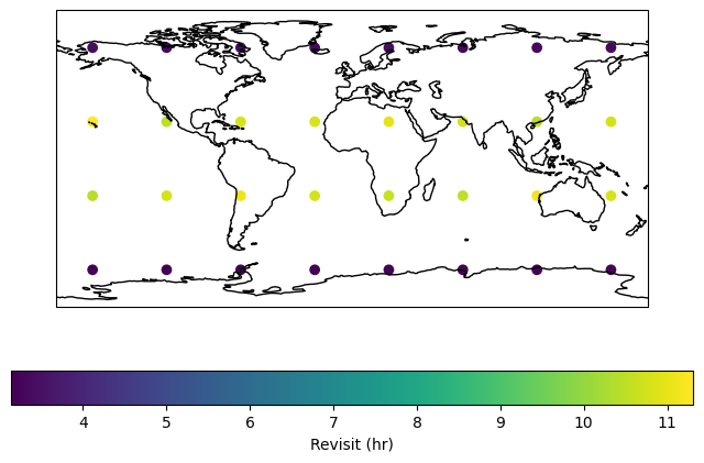
Finally, we can visualize results, first converting metrics to numeric formats.
import matplotlib.pyplot as plt
import cartopy.crs as ccrs

reduced_results["revisit_hr"] = reduced_results.revisit / timedelta(hours=1)

fig, ax = plt.subplots(figsize=(8, 5), subplot_kw={"projection": ccrs.PlateCarree()})
reduced_results.plot(
    column="revisit_hr",
    cmap="viridis",
    legend=True,
    legend_kwds={"label": "Revisit (hr)", "orientation": "horizontal"},
    ax=ax,
    transform=ccrs.PlateCarree()
)
ax.coastlines()
ax.set_global()
plt.show()
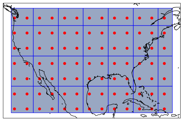
Coverage analyses can also be aggregated to spatial regions for improved visualizations. This example focuses on a smaller spatial region covering the Continental United States (CONUS) defined by a Polygon. Similar to how the generate_equally_spaced_points generates uniformly-distributed points (in latitude/longitude), the function generate_equally_spaced_cells generates uniformly distributed cells. This example uses twice the characteristic distance (1000 km vs. 500 km) such that each cell covers about four points.
from shapely.geometry import Polygon

target = Polygon([(-125, 50), (-67, 50), (-67, 19), (-125, 19), (-125, 50)])

import geopandas as gpd

target_area = gpd.GeoDataFrame({"geometry": target}, index=[0], crs="EPSG:4326")

from tatc.generation.points import generate_equally_spaced_points
from tatc.generation.cells import generate_equally_spaced_cells

points_df = generate_equally_spaced_points(500e3, mask=target)
cells_df = generate_equally_spaced_cells(1000e3, mask=target)

display(cells_df)

import matplotlib.pyplot as plt
import cartopy.crs as ccrs

fig, ax = plt.subplots(figsize=(8, 5), subplot_kw={"projection": ccrs.PlateCarree()})
target_area.plot(alpha=0.5, ax=ax, transform=ccrs.PlateCarree())
points_df.plot(color="r", ax=ax, transform=ccrs.PlateCarree())
cells_df.plot(edgecolor="b", facecolor=(1, 0, 0, 0.1), ax=ax, transform=ccrs.PlateCarree())
ax.coastlines()
plt.show()
| cell_id | geometry | |
|---|---|---|
| 0 | 486 | POLYGON Z ((-125 19 0, -125 26.91165 0, -117.0... |
| 1 | 487 | POLYGON Z ((-117.04757 19 0, -117.04757 26.911... |
| 2 | 488 | POLYGON Z ((-108.05437 19 0, -108.05437 26.911... |
| 3 | 489 | POLYGON Z ((-99.06117 19 0, -99.06117 26.91165... |
| 4 | 526 | POLYGON Z ((-125 26.91165 0, -125 35.90485 0, ... |
| 5 | 527 | POLYGON Z ((-117.04757 26.91165 0, -117.04757 ... |
| 6 | 528 | POLYGON Z ((-108.05437 26.91165 0, -108.05437 ... |
| 7 | 529 | POLYGON Z ((-99.06117 26.91165 0, -99.06117 35... |
| 8 | 566 | POLYGON Z ((-125 35.90485 0, -125 44.89806 0, ... |
| 9 | 567 | POLYGON Z ((-117.04757 35.90485 0, -117.04757 ... |
| 10 | 490 | POLYGON Z ((-90.06796 19 0, -90.06796 26.91165... |
| 11 | 491 | POLYGON Z ((-81.07476 19 0, -81.07476 26.91165... |
| 12 | 492 | POLYGON Z ((-72.08156 19 0, -72.08156 26.91165... |
| 13 | 530 | POLYGON Z ((-90.06796 26.91165 0, -90.06796 35... |
| 14 | 531 | POLYGON Z ((-81.07476 26.91165 0, -81.07476 35... |
| 15 | 532 | POLYGON Z ((-72.08156 26.91165 0, -72.08156 35... |
| 16 | 569 | POLYGON Z ((-99.06117 35.90485 0, -99.06117 44... |
| 17 | 570 | POLYGON Z ((-90.06796 35.90485 0, -90.06796 44... |
| 18 | 571 | POLYGON Z ((-81.07476 35.90485 0, -81.07476 44... |
| 19 | 572 | POLYGON Z ((-72.08156 35.90485 0, -72.08156 44... |
| 20 | 568 | POLYGON Z ((-108.05437 35.90485 0, -108.05437 ... |
| 21 | 606 | POLYGON Z ((-125 44.89806 0, -125 50 0, -117.0... |
| 22 | 607 | POLYGON Z ((-117.04757 44.89806 0, -117.04757 ... |
| 23 | 608 | POLYGON Z ((-108.05437 44.89806 0, -108.05437 ... |
| 24 | 609 | POLYGON Z ((-99.06117 44.89806 0, -99.06117 50... |
| 25 | 610 | POLYGON Z ((-90.06796 44.89806 0, -90.06796 50... |
| 26 | 611 | POLYGON Z ((-81.07476 44.89806 0, -81.07476 50... |
| 27 | 612 | POLYGON Z ((-72.08156 44.89806 0, -72.08156 50... |
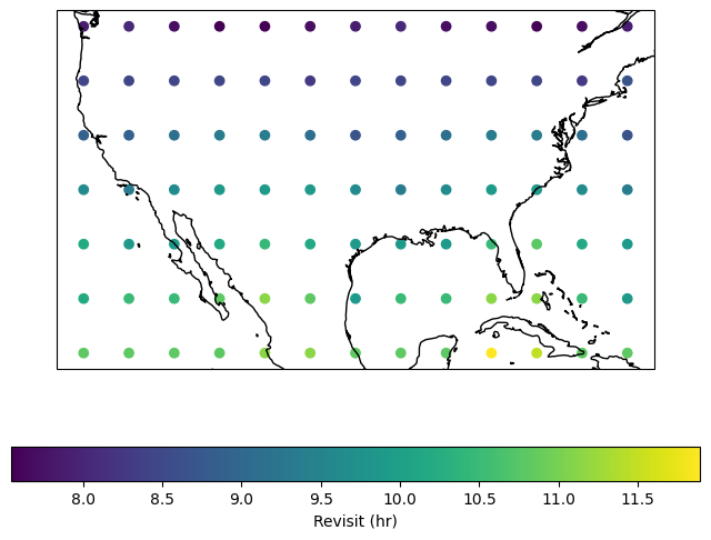
Similar to the prior case, coverage analysis can be performed for each point.
from tatc.schemas import Point

points = points_df.apply(
    lambda r: Point(id=r.point_id, latitude=r.geometry.y, longitude=r.geometry.x),
    axis=1,
)

from joblib import Parallel, delayed
from tatc.analysis.coverage import collect_observations

results_list = Parallel(n_jobs=-1)(
    delayed(collect_observations)(point, noaa20, start, end) for point in points
)
results = pd.concat(results_list, ignore_index=True)

from tatc.analysis import aggregate_observations

aggregated_results = aggregate_observations(results)

from tatc.analysis.coverage import reduce_observations

reduced_results = reduce_observations(aggregated_results)

reduced_results["revisit_hr"] = reduced_results.apply(
    lambda r: r["revisit"] / timedelta(hours=1), axis=1
)

import matplotlib.pyplot as plt
import cartopy.crs as ccrs

fig, ax = plt.subplots(figsize=(8, 6), subplot_kw={"projection": ccrs.PlateCarree()})
reduced_results.plot(
    column="revisit_hr",
    cmap="viridis",
    legend=True,
    legend_kwds={"label": "Revisit (hr)", "orientation": "horizontal"},
    ax=ax,
    transform=ccrs.PlateCarree()
)
ax.coastlines()
plt.show()
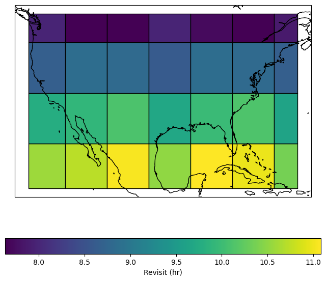
In addition, the results can be merged into the cell specification using a spatial join and dissolve operation. Note that, when working on the reduced results, the revisit aggregation function must perform a weighted average based on the number of samples for each point.
import numpy as np

grid_results = (
    cells_df.sjoin(reduced_results, how="inner", predicate="contains")
    .dissolve(
        by="cell_id",
        aggfunc={
            "samples": "sum",
            "revisit_hr": lambda r: np.average(
                r, weights=reduced_results.loc[r.index, "samples"]
            ),
        },
    )
    .reset_index()
)

import matplotlib.pyplot as plt
import cartopy.crs as ccrs

fig, ax = plt.subplots(figsize=(8, 7), subplot_kw={"projection": ccrs.PlateCarree()})
grid_results.plot(
    column="revisit_hr",
    cmap="viridis",
    edgecolor="k",
    legend=True,
    legend_kwds={"label": "Revisit (hr)", "orientation": "horizontal"},
    ax=ax,
    transform=ccrs.PlateCarree()
)
ax.coastlines()
plt.show()