GNSS Radio Occultation Observations
Global Navigation Satellite System (GNSS) Radio Occultation (RO) samples the environment by observing changes to GNSS signals as the pass through the Earth’s atmosphere. This TAT-C analysis function models when and where GNSS-RO observations can be sampled at the tangent point between a receiver and transmitter, i.e., point along the line-of-sight with minimum distance to the geocenter. This analysis does not consider atmospheric refraction, therefore represents only a coarse estimate of GNSS-RO observations suitable for early-stage mission analysis.
Mathematical Basis
Transmitter/Receiver Geometry
Assume the transmitter (tx) and receiver (rx) have positions \(x_{tx}\) and \(x_{rx}\) and velocities \(v_{tx}\) and \(v_{rx}\), respectively, in a geocentric inertial frame. The transmitter has position \(x_{rx,tx}=x_{tx}-x_{rx}\) and velocity \(v_{rx,tx}=v_{tx}-v_{rx}\) relative to the receiver.
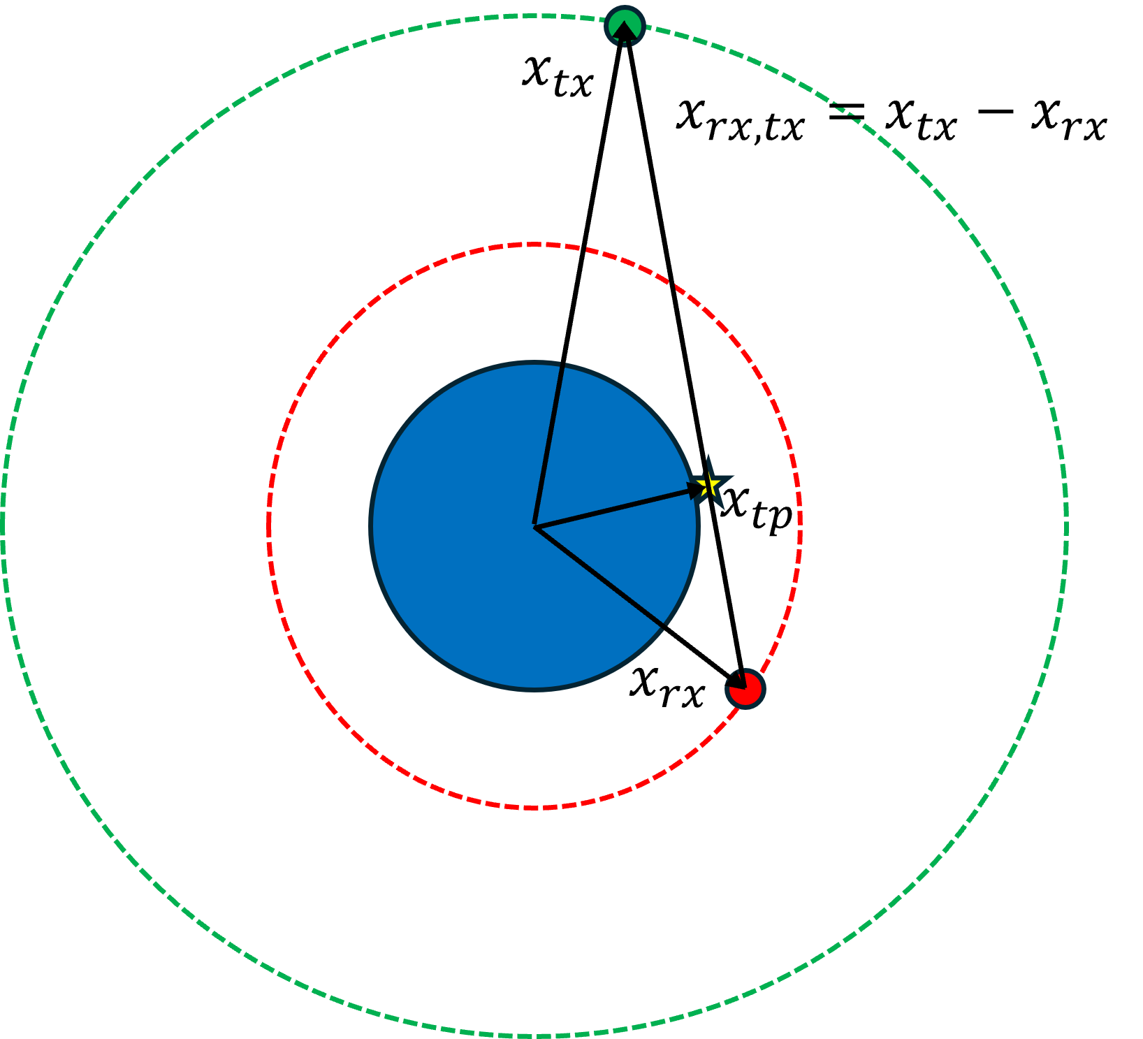
The tangent point has position (via vector geometry):
\(x_{tp} = x_{tx} - \left(x_{tx} \cdot \frac{x_{rx,tx}}{||x_{rx,tx}||}\right) x_{rx,tx}\)
and velocity (via the chain rule):
\(v_{tp} = \frac{d x_{tp}}{dt} = v_{tx} - \left(x_{tx} \cdot \frac{x_{rx,tx}}{||x_{rx,tx}||}\right) v_{rx,tx} - \left[ \frac{v_{tx} \cdot x_{rx,tx} + x_{tx} + v_{rx,tx}}{||x_{rx,tx}||} - 2\frac{\left(x_{tx}\cdot x_{rx,tx}\right)\left(v_{rx,tx}\cdot x_{rx,tx}\right)}{||x_{rx,tx}||^2} \right] x_{rx,tx}\)
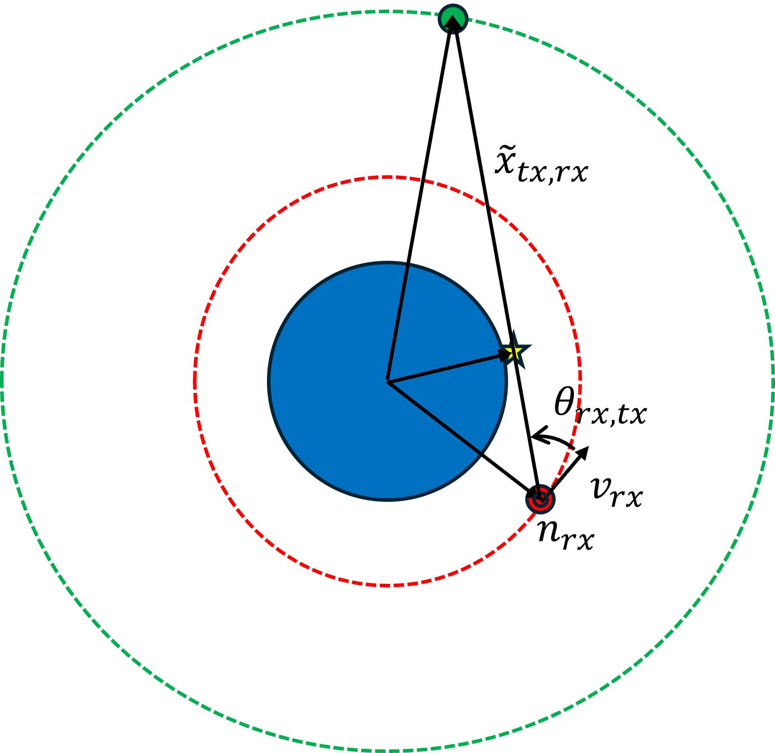
The pitch angle of the transmitter as viewed by the receiver (above/below local horizon) is given by
\(\theta_{rx,tx} = \text{atan2} \left( \tilde{x}_{tx,rx}^n \cdot \frac{x_{rx}}{||x_{rx}||}, \tilde{x}_{tx,rx}^n \cdot \frac{v_{rx}}{||v_{rx}||} \right)\)
where
\(\tilde{x}_{tx,rx}^n = x_{tx,rx} - (n_{rx} \cdot x_{tx,rx}) n_{rx}\)
is the relative transmitter position in the plane normal to the receiver orbit, and
\(n_{rx} = \frac{ x_{rx} \times v_{rx}}{||x_{rx} \times v_{rx}||}\)
is the unit normal to the receiver orbit plane.
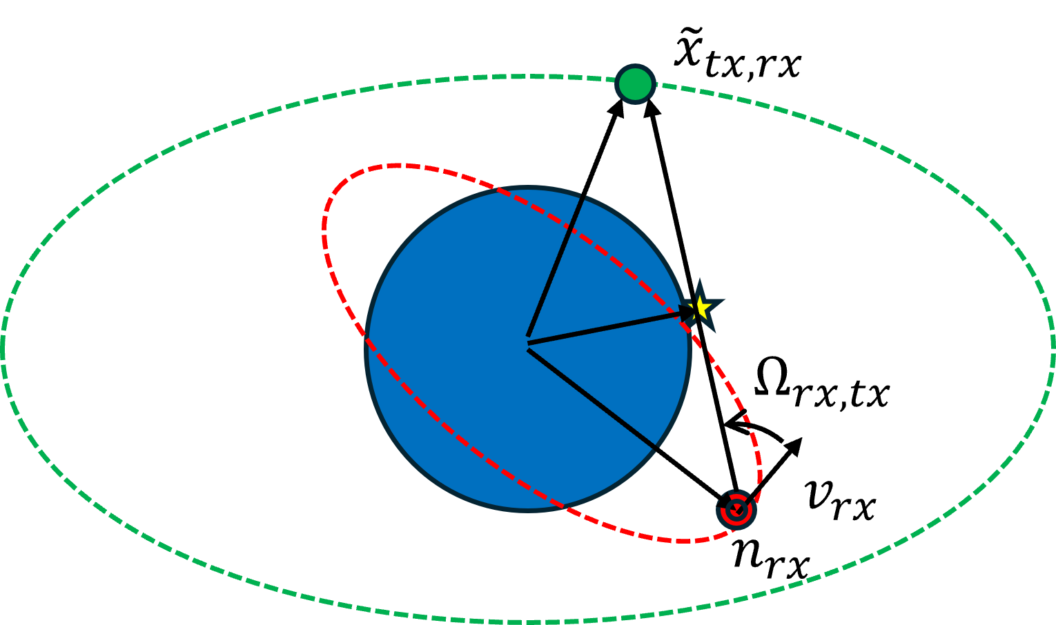
The yaw angle of the transmitter as viewed by the receiver (left/right along local horizontal) is given by
\(\Omega_{rx,tx} = \text{atan2} \left( \tilde{x}_{tx,rx}^t \cdot n_{rx}, \tilde{x}_{tx,rx}^t \cdot \frac{v_{rx}}{||v_{rx}||} \right)\)
where
\(\tilde{x}_{tx,rx}^t = x_{tx,rx} - (\frac{ x_{rx} }{||x_{rx} ||} \cdot x_{tx,rx}) \frac{ x_{rx} }{||x_{rx} ||}\)
is the relative transmitter position in the plane tangent to the receiver orbit.
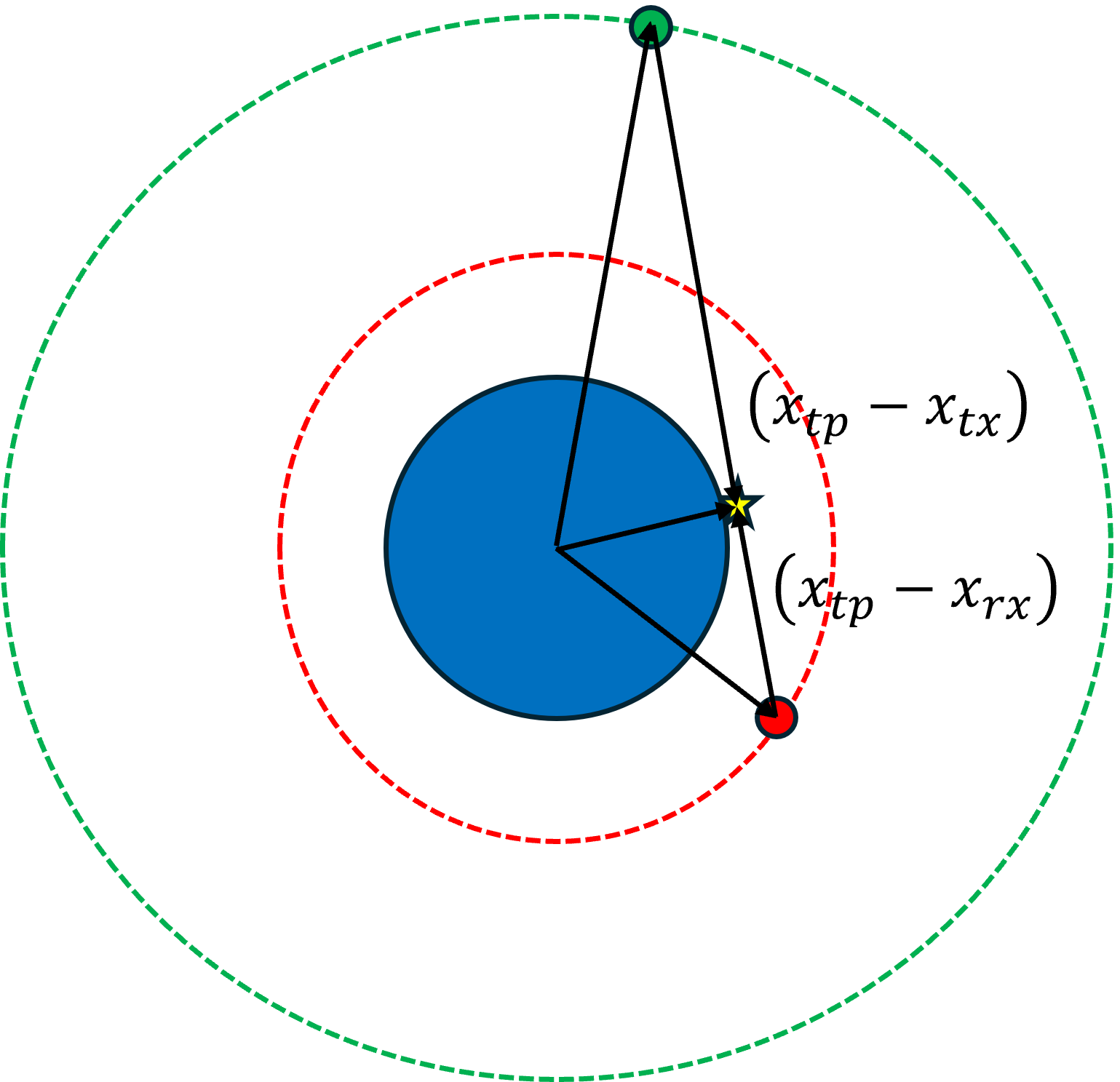
RO Observation Criteria
There are three criteria for a valid RO observation.
First, the tangent point must be between the transmitter and receiver:
\(\text{sgn} \left( (x_{tp} - x_{tx}) \cdot (x_{tp} - x_{rx}) \right) < 0\)
Second, the absolute value yaw angle of the transmitter as viewed by the receiver must be within a maximum bound due to antenna gain patterns:
\(\text{mod}\left( | \Omega_{rx,tx}|, 180 - \Omega_{max} \right) < \Omega_{max}\)
Third, the height of the tangent point must be within a specified range:
\(h_{min} < h < h_{max}\)
where \(h\) is elevation of the tangent point \(x_{tp}\) above a specified geoid such as WGS 84.
Analysis
First, we define scenario configurations. Three parameters set valid GNSS-RO observation conditions between a receiver and transmitter:
max_yawsets the maximum yaw angle (in degrees) between the receiver and transmitter within the receiver’s orbit plane.range_elevationsets the minimum and maximum allowable elevation (in meters) of the tangent point between receiver and transmitter. While realistic GNSS-RO observations sample the atmosphere, a negative minimum value accounts for the lack of refraction considered in this analysis.sample_elevationsets the elevation (in meters) of the tangent point to represent a GNSS-RO observation as a single point, rather than an arc through space.
Other scenario parameters configure the temporal bounds of analysis (start and duration) and set the temporal resolution of orbital motion (time_step).
from datetime import datetime, timedelta, timezone
import numpy as np
# occultation validity constraints
max_yaw = 65 # deg
range_elevation = (-200e3, 60e3) # m
sample_elevation = 0 # m
# scenario configuration
start = datetime(2023, 12, 9, tzinfo=timezone.utc)
time_step = timedelta(seconds=10)
duration = timedelta(hours=1)
times = np.array([start + i * time_step for i in range(duration // time_step)])
Each analysis relies on the definition of a GNSS receiver (e.g., COSMIC-2 FMS) and one or more GNSS transmitters (e.g., the GPS, GLONASS, Galileo, and BeiDou constellations). The code below imports two line elements (TLEs) for each satellite orbit (as of late 2023) and builds a TAT-C Satellite object.
from tatc.schemas import Satellite, TwoLineElements
txs = []
for gnss_dat in ["gps_tle.dat", "glo_tle.dat", "gal_tle.dat", "bei_tle.dat"]:
with open(gnss_dat, "r") as f:
lines = f.read().splitlines()
for i in range(0, len(lines), 3):
txs.append(
Satellite(
name=lines[i], orbit=TwoLineElements(tle=lines[i + 1 : i + 3])
)
)
rx = Satellite(
name="COSMIC-2 FM5",
orbit=TwoLineElements(
tle=[
"1 44358U 19036V 23354.40324524 .00015027 00000-0 91237-3 0 9994",
"2 44358 24.0023 0.0734 0003537 251.0816 108.9304 15.08623759245240",
]
),
)
TAT-C simulates GNSS-RO observations using the collect_ro_observations script. The function propagates the position of the receiver and transmitters and computes the three conditions required for a valid GNSS-RO observation: 1) the tangent point must between the receiver and transmitter, 2) the acute receiver-transmitter azimuth angle must be less than max_azimuth, and 3) the tangent point elevation must be within the range_elevation range.
The outputs report each RO observation including the following fields:
receiver: the receiver satellite nametransmitter: the transmitter satellite nameis_rising: true, if the receiver-transmitter azimuth angle is less thanmax_azimuth(false indicates it is greater than 180 -max_azimuth)geometry: a multipoint geometry that describes the observation arc of points separated bytime_stepposition: a point geometry that describes the observation closest to thesample_elevationvaluerx_tx_azimuth: the transmitter azimuth angle as viewed by the receivertp_tx_azimuth: the transmitter azimuth angle as viewed by the tangent point (i.e., degrees clockwise from North)start: start of the RO observation arcend: end of the RO observation arctime: time of the observation closest to thesample_elevationvalue
from tatc.analysis import collect_ro_observations
ro_obs = collect_ro_observations(
rx, txs, times, sample_elevation, max_yaw, range_elevation
)
display(ro_obs)
| receiver | transmitter | is_rising | geometry | position | rx_tx_pitch | rx_tx_yaw | tp_tx_azimuth | start | end | time | |
|---|---|---|---|---|---|---|---|---|---|---|---|
| 0 | COSMIC-2 FM5 | BEIDOU-3 M7 (C27) | False | MULTIPOINT Z (-0.03172 8.43027 -111422.03599, ... | POINT Z (-0.0317183312985065 8.430274910021483... | -154.829254 | 174.181601 | 298.666783 | 2023-12-09 00:00:00+00:00 | 2023-12-09 00:00:30+00:00 | 2023-12-09 00:00:00+00:00 |
| 1 | COSMIC-2 FM5 | COSMOS 2534 (758) | False | MULTIPOINT Z (8.38669 15.17354 -20482.00391, 8... | POINT Z (8.386687522755755 15.173539678375606 ... | -153.251127 | 148.414002 | 323.957256 | 2023-12-09 00:00:00+00:00 | 2023-12-09 00:01:20+00:00 | 2023-12-09 00:00:00+00:00 |
| 2 | COSMIC-2 FM5 | BEIDOU-3 M12 (C26) | True | MULTIPOINT Z (43.67416 -10.25178 12330.4085, 4... | POINT Z (43.67415791885335 -10.251779478855163... | -22.664009 | 6.514396 | 104.465665 | 2023-12-09 00:00:00+00:00 | 2023-12-09 00:00:20+00:00 | 2023-12-09 00:00:00+00:00 |
| 3 | COSMIC-2 FM5 | COSMOS 2557 (706K) | False | MULTIPOINT Z (5.13858 7.72295 58877.01276, 5.2... | POINT Z (5.509687281172558 7.9175282357802645 ... | -156.574267 | 169.009785 | 304.029604 | 2023-12-09 00:00:20+00:00 | 2023-12-09 00:02:00+00:00 | 2023-12-09 00:00:50+00:00 |
| 4 | COSMIC-2 FM5 | GSAT0215 (PRN E21) | True | MULTIPOINT Z (43.4354 -21.61952 -197994.75109,... | POINT Z (44.94849495030172 -20.81904846996197 ... | -23.893350 | -17.767677 | 126.837457 | 2023-12-09 00:00:10+00:00 | 2023-12-09 00:01:50+00:00 | 2023-12-09 00:01:30+00:00 |
| ... | ... | ... | ... | ... | ... | ... | ... | ... | ... | ... | ... |
| 133 | COSMIC-2 FM5 | BEIDOU-3S M1S (C58) | False | MULTIPOINT Z (-148.06901 -0.43361 47281.53233,... | POINT Z (-146.992685046998 -0.8190136846429314... | -151.471053 | -140.421688 | 212.568932 | 2023-12-09 00:57:50+00:00 | 2023-12-09 00:59:50+00:00 | 2023-12-09 00:58:20+00:00 |
| 134 | COSMIC-2 FM5 | BEIDOU-3 M12 (C26) | False | MULTIPOINT Z (-157.82214 20.0755 44731.25716, ... | POINT Z (-157.66151831979104 20.63188433047461... | -155.288807 | 154.959046 | 271.270420 | 2023-12-09 00:58:10+00:00 | 2023-12-09 00:59:50+00:00 | 2023-12-09 00:58:30+00:00 |
| 135 | COSMIC-2 FM5 | COSMOS 2500 (755) | True | MULTIPOINT Z (-126.69412 44.90944 -194723.7506... | POINT Z (-121.58919915764217 44.59651929331758... | -47.093233 | 63.730350 | 16.239802 | 2023-12-09 00:58:40+00:00 | 2023-12-09 00:59:50+00:00 | 2023-12-09 00:59:50+00:00 |
| 136 | COSMIC-2 FM5 | GSAT0224 (PRN E10) | True | MULTIPOINT Z (-123.55537 45.42334 -193679.7174... | POINT Z (-121.36527296079892 45.17437814841084... | -47.875649 | 63.751499 | 16.226191 | 2023-12-09 00:59:20+00:00 | 2023-12-09 00:59:50+00:00 | 2023-12-09 00:59:50+00:00 |
| 137 | COSMIC-2 FM5 | GPS BIIF-8 (PRN 03) | True | MULTIPOINT Z (-102.06523 18.52248 -194739.9090... | POINT Z (-101.93398093154444 18.83019958019392... | -25.946455 | -11.634382 | 96.639069 | 2023-12-09 00:59:30+00:00 | 2023-12-09 00:59:50+00:00 | 2023-12-09 00:59:50+00:00 |
138 rows × 11 columns
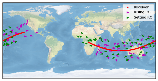
The RO observations can be better visualized by combining with the receiver orbit track.
from tatc.analysis import collect_orbit_track
orbit_track = collect_orbit_track(rx, times)
The resulting plot shows the receiver orbit track and RO observations categorized as rising or setting.
import matplotlib.pyplot as plt
from matplotlib.lines import Line2D
import cartopy.crs as ccrs
fig, ax = plt.subplots(figsize=(10, 4), subplot_kw={"projection": ccrs.PlateCarree()})
orbit_track.plot(ax=ax, marker=".", color="r", lw=0, transform=ccrs.PlateCarree())
ax.quiver(
ro_obs.apply(lambda r: r.position.x, axis=1),
ro_obs.apply(lambda r: r.position.y, axis=1),
ro_obs.apply(lambda r: np.sin(np.radians(r.tp_tx_azimuth)), axis=1),
ro_obs.apply(lambda r: np.cos(np.radians(r.tp_tx_azimuth)), axis=1),
color=ro_obs.apply(lambda r: "m" if r.is_rising else "g", axis=1),
scale=50,
scale_units="width",
transform=ccrs.PlateCarree()
)
ax.stock_img()
ax.set_global()
ax.legend(
handles=[
Line2D([0], [0], marker=".", color="r", lw=0, label="Receiver"),
Line2D([0], [0], marker=">", color="m", lw=0, label="Rising RO"),
Line2D([0], [0], marker=">", color="g", lw=0, label="Setting RO"),
]
)
plt.show()
An animation can show the dynamic collection of RO observations aggregated to individual frames.
import matplotlib.pyplot as plt
import matplotlib.animation as animation
from matplotlib.lines import Line2D
from IPython.display import HTML
from datetime import timedelta
fig, ax = plt.subplots(figsize=(8, 4), subplot_kw={"projection": ccrs.PlateCarree()})
frame_duration = timedelta(minutes=1)
num_frames = int(duration / frame_duration)
def animate(frame):
ax.clear()
time = times[0] + frame * frame_duration
ax.plot(
)
orbit_track.loc[
(orbit_track.time >= time) & (orbit_track.time < time + frame_duration)
].plot(ax=ax, marker=".", color="r", lw=0, transform=ccrs.PlateCarree())
ro_obs_filtered = ro_obs.loc[
(ro_obs.start >= time) & (ro_obs.start < time + frame_duration)
]
if not ro_obs_filtered.empty:
ro_obs_filtered.apply(
lambda r: ax.plot(
[point.x for point in r.geometry.geoms],
[point.y for point in r.geometry.geoms],
".m" if r.is_rising else ".g",
markersize=1,
transform=ccrs.PlateCarree()
),
axis=1,
)
ax.quiver(
ro_obs_filtered.apply(lambda r: r.position.x, axis=1),
ro_obs_filtered.apply(lambda r: r.position.y, axis=1),
ro_obs_filtered.apply(
lambda r: np.sin(np.radians(r.tp_tx_azimuth)), axis=1
),
ro_obs_filtered.apply(
lambda r: np.cos(np.radians(r.tp_tx_azimuth)), axis=1
),
color=ro_obs_filtered.apply(lambda r: "m" if r.is_rising else "g", axis=1),
scale=50,
scale_units="width",
transform=ccrs.PlateCarree()
)
ax.set_global()
ax.coastlines()
ax.set_aspect("equal")
ax.legend(
handles=[
Line2D([0], [0], marker=".", color="r", lw=0, label="Receiver"),
Line2D([0], [0], marker=">", color="m", lw=0, label="Rising RO"),
Line2D([0], [0], marker=">", color="g", lw=0, label="Setting RO"),
]
)
ax.set_title(
time.strftime("%x %X") + "$-$" + (time + frame_duration).strftime("%X")
)
fig.tight_layout()
ani = animation.FuncAnimation(fig, animate, frames=num_frames, interval=200, blit=False)
display(HTML(ani.to_jshtml()))
plt.close()