Compute Coverage
This example demonstrates how to use direct function calls of the low-level TAT-C library to perform coverage analysis over a region of interest.
Similar to the Collect Observations example, the first steps are to define the satellites for the mission. This example again uses the NOAA-20 satellite with a two-line elements model from July 2022 and a VIIRS instrument with field of regard computed based on a 834km altitude and 3000km swath width.
[1]:
from tatc import utils
from tatc.schemas import Instrument, Satellite, TwoLineElements

viirs = Instrument(
    name="VIIRS",
    field_of_regard=utils.swath_width_to_field_of_regard(834000, 3000000),
)
noaa20 = Satellite(
    name="NOAA 20",
    orbit=TwoLineElements(
        tle=[
            "1 43013U 17073A   22195.78278435  .00000038  00000+0  38919-4 0  9996",
            "2 43013  98.7169 133.9110 0001202  63.8768 296.2532 14.19561306241107",
        ]
    ),
    instruments=[viirs],
)
The mission considers a 30-day integration period starting at noon UTC on July 14, 2022.
[2]:
from datetime import datetime, timedelta, timezone

start = datetime(year=2022, month=7, day=14, hour=12, tzinfo=timezone.utc)
end = start + timedelta(days=30)
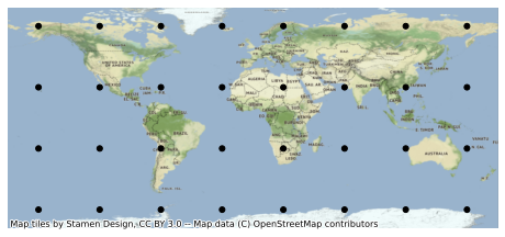
Coverage analyses typically compute metrics over a spatial region. The generate_cubed_sphere_points method in TAT-C distributes sample points over a uniform latitude-longitude grid, scaled based on a characteristic distance, set to 5000 km in this example.
[3]:
from tatc.generation import generate_cubed_sphere_points

points_df = generate_cubed_sphere_points(5000e3)
display(points_df)
| point_id | geometry | |
|---|---|---|
| 0 | 0 | POINT Z (-157.51699 -67.51699 0.00000) |
| 1 | 1 | POINT Z (-112.55097 -67.51699 0.00000) |
| 2 | 2 | POINT Z (-67.58495 -67.51699 0.00000) |
| 3 | 3 | POINT Z (-22.61894 -67.51699 0.00000) |
| 4 | 4 | POINT Z (22.34708 -67.51699 0.00000) |
| 5 | 5 | POINT Z (67.31310 -67.51699 0.00000) |
| 6 | 6 | POINT Z (112.27912 -67.51699 0.00000) |
| 7 | 7 | POINT Z (157.24514 -67.51699 0.00000) |
| 8 | 8 | POINT Z (-157.51699 -22.55097 0.00000) |
| 9 | 9 | POINT Z (-112.55097 -22.55097 0.00000) |
| 10 | 10 | POINT Z (-67.58495 -22.55097 0.00000) |
| 11 | 11 | POINT Z (-22.61894 -22.55097 0.00000) |
| 12 | 12 | POINT Z (22.34708 -22.55097 0.00000) |
| 13 | 13 | POINT Z (67.31310 -22.55097 0.00000) |
| 14 | 14 | POINT Z (112.27912 -22.55097 0.00000) |
| 15 | 15 | POINT Z (157.24514 -22.55097 0.00000) |
| 16 | 16 | POINT Z (-157.51699 22.41505 0.00000) |
| 17 | 17 | POINT Z (-112.55097 22.41505 0.00000) |
| 18 | 18 | POINT Z (-67.58495 22.41505 0.00000) |
| 19 | 19 | POINT Z (-22.61894 22.41505 0.00000) |
| 20 | 20 | POINT Z (22.34708 22.41505 0.00000) |
| 21 | 21 | POINT Z (67.31310 22.41505 0.00000) |
| 22 | 22 | POINT Z (112.27912 22.41505 0.00000) |
| 23 | 23 | POINT Z (157.24514 22.41505 0.00000) |
| 24 | 24 | POINT Z (-157.51699 67.38106 0.00000) |
| 25 | 25 | POINT Z (-112.55097 67.38106 0.00000) |
| 26 | 26 | POINT Z (-67.58495 67.38106 0.00000) |
| 27 | 27 | POINT Z (-22.61894 67.38106 0.00000) |
| 28 | 28 | POINT Z (22.34708 67.38106 0.00000) |
| 29 | 29 | POINT Z (67.31310 67.38106 0.00000) |
| 30 | 30 | POINT Z (112.27912 67.38106 0.00000) |
| 31 | 31 | POINT Z (157.24514 67.38106 0.00000) |
The resulting 32 points are distributed over the globe.
[4]:
import geoplot as gplt
import contextily as ctx

ax = gplt.pointplot(points_df, color="k")
ctx.add_basemap(ax, crs=points_df.crs)
As the TAT-C analysis functions require points specified in the TAT-C format, rather than a data frame, it is often convenient to convert and store the points in a separate list.
[5]:
from tatc.schemas import Point

points = points_df.apply(
    lambda r: Point(id=r.point_id, latitude=r.geometry.y, longitude=r.geometry.x),
    axis=1,
)
The collect_observations method can be called either using sequential or parallel computation (using joblib). While there is some overhead associated with parallel computation, it is usually faster on modern multi-core machines.
[6]:
from tatc.analysis import collect_observations

import time

t = time.time()
results_list = [
    collect_observations(point, noaa20, viirs, start, end) for point in points
]
print(f"Sequential computation completed in {time.time() - t:.2f} seconds")
Sequential computation completed in 10.57 seconds
[7]:
from tatc.analysis import collect_observations

import time
from joblib import Parallel, delayed

t = time.time()
results_list = Parallel(n_jobs=-1)(
    delayed(collect_observations)(point, noaa20, viirs, start, end) for point in points
)
print(f"Parallel computation completed in {time.time() - t:.2f} seconds")
Parallel computation completed in 4.44 seconds
Next, we concatenate the results into a single data frame.
[8]:
import pandas as pd

results = pd.concat(results_list, ignore_index=True)
display(results)
| point_id | geometry | satellite | instrument | start | end | epoch | sat_alt | sat_az | |
|---|---|---|---|---|---|---|---|---|---|
| 0 | 0 | POINT Z (-157.51699 -67.51699 0.00000) | NOAA 20 | VIIRS | 2022-07-14 23:30:13.504937+00:00 | 2022-07-14 23:35:24.700151+00:00 | 2022-07-14 23:32:49.102544+00:00 | 30.035319 | 90.532033 |
| 1 | 0 | POINT Z (-157.51699 -67.51699 0.00000) | NOAA 20 | VIIRS | 2022-07-15 01:09:57.221103+00:00 | 2022-07-15 01:17:36.070193+00:00 | 2022-07-15 01:13:46.645648+00:00 | 84.027201 | 71.176629 |
| 2 | 0 | POINT Z (-157.51699 -67.51699 0.00000) | NOAA 20 | VIIRS | 2022-07-15 02:50:32.021280+00:00 | 2022-07-15 02:56:59.202403+00:00 | 2022-07-15 02:53:45.611841500+00:00 | 41.004603 | 223.802850 |
| 3 | 0 | POINT Z (-157.51699 -67.51699 0.00000) | NOAA 20 | VIIRS | 2022-07-15 04:31:23.154019+00:00 | 2022-07-15 04:34:35.637143+00:00 | 2022-07-15 04:32:59.395581+00:00 | 23.798801 | 200.198288 |
| 4 | 0 | POINT Z (-157.51699 -67.51699 0.00000) | NOAA 20 | VIIRS | 2022-07-15 07:48:30.230323+00:00 | 2022-07-15 07:52:58.807543+00:00 | 2022-07-15 07:50:44.518933+00:00 | 27.400102 | 151.773103 |
| ... | ... | ... | ... | ... | ... | ... | ... | ... | ... |
| 4782 | 31 | POINT Z (157.24514 67.38106 0.00000) | NOAA 20 | VIIRS | 2022-08-12 18:28:49.325939+00:00 | 2022-08-12 18:34:03.183661+00:00 | 2022-08-12 18:31:26.254800+00:00 | 31.260813 | 324.671157 |
| 4783 | 31 | POINT Z (157.24514 67.38106 0.00000) | NOAA 20 | VIIRS | 2022-08-12 21:48:42.817756+00:00 | 2022-08-12 21:49:48.545180+00:00 | 2022-08-12 21:49:15.681468+00:00 | 21.116289 | 13.096140 |
| 4784 | 31 | POINT Z (157.24514 67.38106 0.00000) | NOAA 20 | VIIRS | 2022-08-12 23:25:35.417650+00:00 | 2022-08-12 23:31:03.448822+00:00 | 2022-08-12 23:28:19.433236+00:00 | 32.782441 | 37.026059 |
| 4785 | 31 | POINT Z (157.24514 67.38106 0.00000) | NOAA 20 | VIIRS | 2022-08-13 01:04:19.959524+00:00 | 2022-08-13 01:11:46.499770+00:00 | 2022-08-13 01:08:03.229647+00:00 | 73.846580 | 59.292237 |
| 4786 | 31 | POINT Z (157.24514 67.38106 0.00000) | NOAA 20 | VIIRS | 2022-08-13 02:45:30.353434+00:00 | 2022-08-13 02:51:54.566357+00:00 | 2022-08-13 02:48:42.459895500+00:00 | 40.295326 | 263.804774 |
4787 rows × 9 columns
The aggregate_observations function computes the access and revisit statistics for each point.
[9]:
from tatc.analysis import aggregate_observations

aggregated_results = aggregate_observations(results)
display(aggregated_results)
| geometry | point_id | satellite | instrument | start | epoch | end | access | revisit | |
|---|---|---|---|---|---|---|---|---|---|
| 0 | POINT Z (-157.51699 -67.51699 0.00000) | 0 | NOAA 20 | VIIRS | 2022-07-14 23:30:13.504937+00:00 | 2022-07-14 23:32:49.102543872+00:00 | 2022-07-14 23:35:24.700151+00:00 | 0 days 00:05:11.195214 | NaT |
| 1 | POINT Z (-157.51699 -67.51699 0.00000) | 0 | NOAA 20 | VIIRS | 2022-07-15 01:09:57.221103+00:00 | 2022-07-15 01:13:46.645647872+00:00 | 2022-07-15 01:17:36.070193+00:00 | 0 days 00:07:38.849090 | 0 days 01:34:32.520952 |
| 2 | POINT Z (-157.51699 -67.51699 0.00000) | 0 | NOAA 20 | VIIRS | 2022-07-15 02:50:32.021280+00:00 | 2022-07-15 02:53:45.611841536+00:00 | 2022-07-15 02:56:59.202403+00:00 | 0 days 00:06:27.181123 | 0 days 01:32:55.951087 |
| 3 | POINT Z (-157.51699 -67.51699 0.00000) | 0 | NOAA 20 | VIIRS | 2022-07-15 04:31:23.154019+00:00 | 2022-07-15 04:32:59.395580928+00:00 | 2022-07-15 04:34:35.637143+00:00 | 0 days 00:03:12.483124 | 0 days 01:34:23.951616 |
| 4 | POINT Z (-157.51699 -67.51699 0.00000) | 0 | NOAA 20 | VIIRS | 2022-07-15 07:48:30.230323+00:00 | 2022-07-15 07:50:44.518932992+00:00 | 2022-07-15 07:52:58.807543+00:00 | 0 days 00:04:28.577220 | 0 days 03:13:54.593180 |
| ... | ... | ... | ... | ... | ... | ... | ... | ... | ... |
| 4782 | POINT Z (157.24514 67.38106 0.00000) | 31 | NOAA 20 | VIIRS | 2022-08-12 18:28:49.325939+00:00 | 2022-08-12 18:31:26.254799872+00:00 | 2022-08-12 18:34:03.183661+00:00 | 0 days 00:05:13.857722 | 0 days 01:33:21.770501 |
| 4783 | POINT Z (157.24514 67.38106 0.00000) | 31 | NOAA 20 | VIIRS | 2022-08-12 21:48:42.817756+00:00 | 2022-08-12 21:49:15.681467904+00:00 | 2022-08-12 21:49:48.545180+00:00 | 0 days 00:01:05.727424 | 0 days 03:14:39.634095 |
| 4784 | POINT Z (157.24514 67.38106 0.00000) | 31 | NOAA 20 | VIIRS | 2022-08-12 23:25:35.417650+00:00 | 2022-08-12 23:28:19.433235968+00:00 | 2022-08-12 23:31:03.448822+00:00 | 0 days 00:05:28.031172 | 0 days 01:35:46.872470 |
| 4785 | POINT Z (157.24514 67.38106 0.00000) | 31 | NOAA 20 | VIIRS | 2022-08-13 01:04:19.959524+00:00 | 2022-08-13 01:08:03.229647104+00:00 | 2022-08-13 01:11:46.499770+00:00 | 0 days 00:07:26.540246 | 0 days 01:33:16.510702 |
| 4786 | POINT Z (157.24514 67.38106 0.00000) | 31 | NOAA 20 | VIIRS | 2022-08-13 02:45:30.353434+00:00 | 2022-08-13 02:48:42.459895552+00:00 | 2022-08-13 02:51:54.566357+00:00 | 0 days 00:06:24.212923 | 0 days 01:33:43.853664 |
4787 rows × 9 columns
The reduce_observations function computes descriptive statistics for each point.
[10]:
from tatc.analysis import reduce_observations

reduced_results = reduce_observations(aggregated_results)
display(reduced_results)
| point_id | geometry | access | revisit | samples | |
|---|---|---|---|---|---|
| 0 | 0 | POINT Z (-157.51699 -67.51699 0.00000) | 0 days 00:05:28.705247 | 0 days 02:56:33.403049 | 234 |
| 1 | 1 | POINT Z (-112.55097 -67.51699 0.00000) | 0 days 00:05:27.187784 | 0 days 02:55:27.374120 | 236 |
| 2 | 2 | POINT Z (-67.58495 -67.51699 0.00000) | 0 days 00:05:28.226225 | 0 days 02:55:47.326095 | 235 |
| 3 | 3 | POINT Z (-22.61894 -67.51699 0.00000) | 0 days 00:05:28.703592 | 0 days 02:56:12.255015 | 235 |
| 4 | 4 | POINT Z (22.34708 -67.51699 0.00000) | 0 days 00:05:29.869214 | 0 days 02:57:19.324365 | 233 |
| 5 | 5 | POINT Z (67.31310 -67.51699 0.00000) | 0 days 00:05:26.638983 | 0 days 02:57:41.792189 | 236 |
| 6 | 6 | POINT Z (112.27912 -67.51699 0.00000) | 0 days 00:05:29.207116 | 0 days 02:58:25.816311 | 235 |
| 7 | 7 | POINT Z (157.24514 -67.51699 0.00000) | 0 days 00:05:29.089517 | 0 days 02:59:13.646230 | 234 |
| 8 | 8 | POINT Z (-157.51699 -22.55097 0.00000) | 0 days 00:05:48.303140 | 0 days 09:52:38.681883 | 72 |
| 9 | 9 | POINT Z (-112.55097 -22.55097 0.00000) | 0 days 00:05:52.743758 | 0 days 10:01:06.235517 | 71 |
| 10 | 10 | POINT Z (-67.58495 -22.55097 0.00000) | 0 days 00:05:58.830235 | 0 days 10:08:21.257912 | 70 |
| 11 | 11 | POINT Z (-22.61894 -22.55097 0.00000) | 0 days 00:05:53.433621 | 0 days 10:01:05.661949 | 71 |
| 12 | 12 | POINT Z (22.34708 -22.55097 0.00000) | 0 days 00:05:45.642137 | 0 days 09:51:37.182239 | 71 |
| 13 | 13 | POINT Z (67.31310 -22.55097 0.00000) | 0 days 00:05:51.746116 | 0 days 09:53:37.228465 | 72 |
| 14 | 14 | POINT Z (112.27912 -22.55097 0.00000) | 0 days 00:06:01.018137 | 0 days 10:09:25.218953 | 70 |
| 15 | 15 | POINT Z (157.24514 -22.55097 0.00000) | 0 days 00:05:58.445041 | 0 days 10:10:53.365711 | 70 |
| 16 | 16 | POINT Z (-157.51699 22.41505 0.00000) | 0 days 00:06:03.724390 | 0 days 10:28:18.609280 | 69 |
| 17 | 17 | POINT Z (-112.55097 22.41505 0.00000) | 0 days 00:05:45.936852 | 0 days 09:53:43.729175 | 72 |
| 18 | 18 | POINT Z (-67.58495 22.41505 0.00000) | 0 days 00:05:51.188100 | 0 days 10:11:01.776398 | 70 |
| 19 | 19 | POINT Z (-22.61894 22.41505 0.00000) | 0 days 00:05:53.721279 | 0 days 10:10:58.296466 | 70 |
| 20 | 20 | POINT Z (22.34708 22.41505 0.00000) | 0 days 00:05:56.431973 | 0 days 10:10:18.485633 | 71 |
| 21 | 21 | POINT Z (67.31310 22.41505 0.00000) | 0 days 00:05:53.187639 | 0 days 10:09:53.996686 | 70 |
| 22 | 22 | POINT Z (112.27912 22.41505 0.00000) | 0 days 00:05:43.524953 | 0 days 09:52:43.535228 | 72 |
| 23 | 23 | POINT Z (157.24514 22.41505 0.00000) | 0 days 00:05:50.324973 | 0 days 10:01:08.941317 | 71 |
| 24 | 24 | POINT Z (-157.51699 67.38106 0.00000) | 0 days 00:05:32.508810 | 0 days 03:10:32.061516 | 221 |
| 25 | 25 | POINT Z (-112.55097 67.38106 0.00000) | 0 days 00:05:30.892440 | 0 days 03:09:40.755148 | 222 |
| 26 | 26 | POINT Z (-67.58495 67.38106 0.00000) | 0 days 00:05:33.057176 | 0 days 03:10:31.072390 | 220 |
| 27 | 27 | POINT Z (-22.61894 67.38106 0.00000) | 0 days 00:05:30.675408 | 0 days 03:09:40.962655 | 222 |
| 28 | 28 | POINT Z (22.34708 67.38106 0.00000) | 0 days 00:05:29.730143 | 0 days 03:08:48.883590 | 223 |
| 29 | 29 | POINT Z (67.31310 67.38106 0.00000) | 0 days 00:05:30.703513 | 0 days 03:06:51.457476 | 222 |
| 30 | 30 | POINT Z (112.27912 67.38106 0.00000) | 0 days 00:05:27.964761 | 0 days 03:05:10.758904 | 224 |
| 31 | 31 | POINT Z (157.24514 67.38106 0.00000) | 0 days 00:05:29.196438 | 0 days 03:06:00.960764 | 223 |
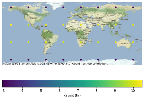
Finally, we can visualize results, first converting metrics to numeric formats.
[11]:
import geoplot as gplt
import contextily as ctx

reduced_results["revisit_hr"] = reduced_results.revisit / timedelta(hours=1)
ax = gplt.pointplot(
    reduced_results,
    hue="revisit_hr",
    legend=True,
    legend_kwargs={"label": "Revisit (hr)", "orientation": "horizontal"},
)
ctx.add_basemap(ax, crs=reduced_results.crs)
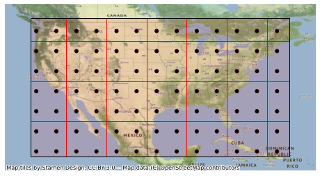
Coverage analyses can also be aggregated to spatial regions for improved visualizations. This example focuses on a smaller spatial region covering the Continental United States (CONUS) defined by a Polygon. Similar to how the generate_cubed_sphere_points generates uniformly-distributed points (in latitude/longitude), the function generate_cubed_sphere_cells generates uniformly distributed cells. This example uses twice the characteristic distance (1000 km vs. 500 km) such that each cell
covers about four points.
[12]:
from shapely.geometry import Polygon

target = Polygon([(-125, 50), (-67, 50), (-67, 19), (-125, 19), (-125, 50)])

import geopandas as gpd

target_area = gpd.GeoDataFrame({"geometry": target}, index=[0], crs="EPSG:4326")

from tatc.generation.points import generate_cubed_sphere_points
from tatc.generation.cells import generate_cubed_sphere_cells

points_df = generate_cubed_sphere_points(500e3, mask=target)
cells_df = generate_cubed_sphere_cells(1000e3, mask=target)

display(cells_df)

import geoplot as gplt
import contextily as ctx

ax = gplt.pointplot(points_df, color="k")
gplt.polyplot(cells_df, ax=ax, edgecolor="r", facecolor=(1, 0, 0, 0.1), zorder=1)
gplt.polyplot(target_area, ax=ax, zorder=2)
ctx.add_basemap(
    ax,
    crs=points_df.crs,
)
| cell_id | geometry | |
|---|---|---|
| 0 | 486 | POLYGON Z ((-125.00000 19.00000 0.00000, -125.... |
| 1 | 526 | POLYGON Z ((-125.00000 26.91165 0.00000, -125.... |
| 2 | 566 | POLYGON Z ((-125.00000 35.90485 0.00000, -125.... |
| 3 | 606 | POLYGON Z ((-125.00000 44.89806 0.00000, -125.... |
| 4 | 487 | POLYGON Z ((-117.04757 19.00000 0.00000, -117.... |
| 5 | 527 | POLYGON Z ((-117.04757 26.91165 0.00000, -117.... |
| 6 | 567 | POLYGON Z ((-117.04757 35.90485 0.00000, -117.... |
| 7 | 607 | POLYGON Z ((-117.04757 44.89806 0.00000, -117.... |
| 8 | 488 | POLYGON Z ((-108.05437 19.00000 0.00000, -108.... |
| 9 | 528 | POLYGON Z ((-108.05437 26.91165 0.00000, -108.... |
| 10 | 568 | POLYGON Z ((-108.05437 35.90485 0.00000, -108.... |
| 11 | 608 | POLYGON Z ((-108.05437 44.89806 0.00000, -108.... |
| 12 | 489 | POLYGON Z ((-99.06117 19.00000 0.00000, -99.06... |
| 13 | 529 | POLYGON Z ((-99.06117 26.91165 0.00000, -99.06... |
| 14 | 569 | POLYGON Z ((-99.06117 35.90485 0.00000, -99.06... |
| 15 | 609 | POLYGON Z ((-99.06117 44.89806 0.00000, -99.06... |
| 16 | 490 | POLYGON Z ((-90.06796 19.00000 0.00000, -90.06... |
| 17 | 530 | POLYGON Z ((-90.06796 26.91165 0.00000, -90.06... |
| 18 | 570 | POLYGON Z ((-90.06796 35.90485 0.00000, -90.06... |
| 19 | 610 | POLYGON Z ((-90.06796 44.89806 0.00000, -90.06... |
| 20 | 491 | POLYGON Z ((-81.07476 19.00000 0.00000, -81.07... |
| 21 | 531 | POLYGON Z ((-81.07476 26.91165 0.00000, -81.07... |
| 22 | 571 | POLYGON Z ((-81.07476 35.90485 0.00000, -81.07... |
| 23 | 611 | POLYGON Z ((-81.07476 44.89806 0.00000, -81.07... |
| 24 | 492 | POLYGON Z ((-72.08156 19.00000 0.00000, -72.08... |
| 25 | 532 | POLYGON Z ((-72.08156 26.91165 0.00000, -72.08... |
| 26 | 572 | POLYGON Z ((-72.08156 35.90485 0.00000, -72.08... |
| 27 | 612 | POLYGON Z ((-72.08156 44.89806 0.00000, -72.08... |
Similar to the prior case, coverage analysis can be performed for each point.
[13]:
from tatc.schemas import Point

points = points_df.apply(
    lambda r: Point(id=r.point_id, latitude=r.geometry.y, longitude=r.geometry.x),
    axis=1,
)

from joblib import Parallel, delayed
from tatc.analysis.coverage import collect_observations

results_list = Parallel(n_jobs=-1)(
    delayed(collect_observations)(point, noaa20, viirs, start, end) for point in points
)
results = pd.concat(results_list, ignore_index=True)

from tatc.analysis import aggregate_observations

aggregated_results = aggregate_observations(results)

from tatc.analysis.coverage import reduce_observations

reduced_results = reduce_observations(aggregated_results)

import geoplot as gplt
import contextily as ctx

reduced_results["revisit_hr"] = reduced_results.apply(
    lambda r: r["revisit"] / timedelta(hours=1), axis=1
)
ax = gplt.pointplot(
    reduced_results,
    hue="revisit_hr",
    legend=True,
    legend_kwargs={"label": "Revisit (hr)", "orientation": "horizontal"},
)
ctx.add_basemap(
    ax,
    crs=reduced_results.crs,
)
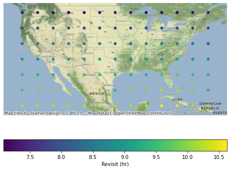
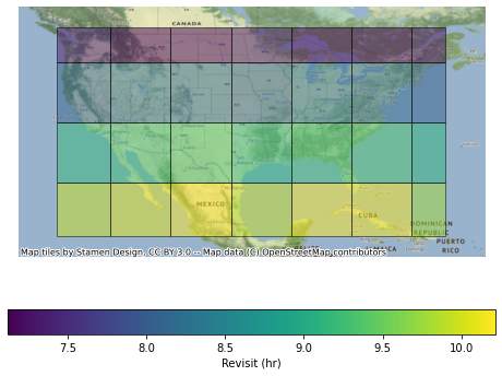
In addition, the results can be merged into the cell specification using a spatial join and dissolve operation. Note that, when working on the reduced results, the revisit aggregation function must perform a weighted average based on the number of samples for each point.
[14]:
import numpy as np

grid_results = (
    cells_df.sjoin(reduced_results, how="inner", predicate="contains")
    .dissolve(
        by="cell_id",
        aggfunc={
            "samples": "sum",
            "revisit_hr": lambda r: np.average(
                r, weights=reduced_results.loc[r.index, "samples"]
            ),
        },
    )
    .reset_index()
)

import geoplot as gplt
import contextily as ctx

ax = gplt.choropleth(
    grid_results,
    hue="revisit_hr",
    alpha=0.5,
    legend=True,
    legend_kwargs={"label": "Revisit (hr)", "orientation": "horizontal"},
)
ctx.add_basemap(
    ax,
    crs=reduced_results.crs,
)